


Design IIR Filters Using Cascaded Biquads
This article shows how to implement a Butterworth IIR lowpass filter as a cascade of second-order IIR filters, or biquads. We’ll derive how to calculate the coefficients of the biquads and do some examples using a Matlab function biquad_synth provided in the Appendix. Although we’ll be designing Butterworth filters, the approach applies to any all-pole lowpass filter (Chebyshev, Bessel, etc). As we’ll see, the cascaded-biquad design is less sensitive to coefficient quantization than a single high-order IIR, particularly for lower cut-off frequencies [1, 2]
In an earlier post on IIR Butterworth lowpass filters [3], I presented the pole-zero form of the lowpass response H(z) as follows:
$$H(z)=K\frac{(z+1)^N}{(z-p_1)(z-p_2)...(z-p_N)}\qquad(1)$$
The N zeros at z = 1 (ω= π or f = fs/2) occur when we transform the lowpass analog zeros from the s-domain to z-domain using the bilinear transform. Our goal is to convert H(z) into a cascade of second-order sections. If we stipulate that N is even, then we can write H(z) as:
$H(z)=K_1\frac{(z+1)^2}{(z-p_1)(z-p_2)}\cdot K_2\frac{(z+1)^2}{(z-p_3)(z-p_4)}\cdot...\cdot K_{N/2}\frac{(z+1)^2}{(z-p_{N-1})(z-p_N)} \qquad(2)$
Each term in equation 2 is biquadratic – it has quadratic numerator and denominator. It is not necessary to use a separate gain K for each term; we could also use just a single gain for the whole cascade.
The filter is even order, so all poles occur in complex-conjugate pairs. We’ll assign a complex-conjugate pole pair to the denominator of each term of equation 2. We can then write each term as:
$$H_k(z)=K_k\frac{(z+1)^2}{(z-p_k)(z-p^*_k)},\quad k=1:N/2$$
where $p^*_k$ is the complex conjugate of $p_k$. Expanding the numerator and denominator, we get:
$$H_k(z)=K_k\frac{z^2+2z+1}{z^2+a_1z+a_2}$$
where a1= -2*real(pk) and a2= |pk|2. Dividing numerator and denominator by z2, we get:
$$H_k(z)=K_k\frac{1+2z^{-1}+z^{-2}}{1+a_1z^{-1}+a_2z^{-2}}\qquad(3)$$
We want the gain of each biquad section to equal 1 at ω=0. Letting $z= e^{jω}$, we have z= 1. Then:
$$H_k(z)=1=K_k\frac{\sum{b}}{\sum{a}}$$
so
$$K_k=\frac{\sum{a}}{4}\qquad(4)$$
where a = [1 a1 a2] are the denominator coefficients of the biquad section. Summarizing the coefficient values, we have:
b = [1 2 1]
a= [1 -2*real(pk) |pk|2]
$K= \sum{a}/4$
A biquad lowpass block diagram using the Direct form II
structure [4,5] is shown in Figure 1. We
will cascade N/2 biquads to implement an N
th order filter (N
even). Note that the feed-forward
coefficients b have the same value for all N/2 biquads in a filter. This is evident from Equation 3.
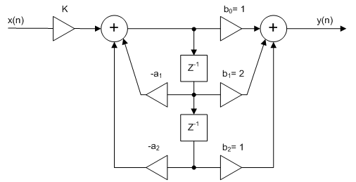
Figure 1 Biquad (second-order) lowpass all-pole filter
Direct form II
Example
In this example, we’ll use biquad_synth to design a 6th order Butterworth lowpass filter with -3 dB frequency of 15 Hz and fs= 100 Hz. Note biquad_synth uses the bilinear transform with prewarping [3] to transform H(s) to H(z). The filter will consist of three biquads, as shown in Figure 2. biquad_synth computes the denominator (feedback) coefficients a of each biquad. The gains K are computed separately. Note biquad_synth contains code developed in an earlier post on IIR Butterworth filter synthesis [3]. Here is the function call and the function output:
    N= 6;       % filter order
    fc= 15;     % Hz  -3 dB frequency
    fs= 100;    % Hz  sample frequency
    a= biquad_synth(N,fc,fs)
    a =
        1.0000   -0.6599    0.1227
        1.0000   -0.7478    0.2722
        1.0000   -0.9720    0.6537
Each row of the matrix a contains the denominator coefficients of a biquad. As we already determined, the numerator coefficients b are the same for all three biquads:
b= [1 2 1];The gains for each biquad are, from equation 4:
    K1= sum(a(1,:)/4;
    K2= sum(a(2,:)/4;
    K3= sum(a(3,:)/4;
Now
we can compute the frequency response of each biquad. The overall response is their product.
    [h1,f] = freqz(K1*b,a(1,:),512,fs);
    [h2,f] = freqz(K2*b,a(2,:),512,fs);
    [h3,f] = freqz(K3*b,a(3,:),512,fs);
    h= abs(h1.*h2.*h3);
    H= 20*log10(abs(h));
The magnitude response of each biquad and the overall
response are plotted in Figure 3. The
sequence of the biquads doesn’t matter in theory; however, placing the biquad
with the peaking response (h3) last minimizes the chance of clipping.
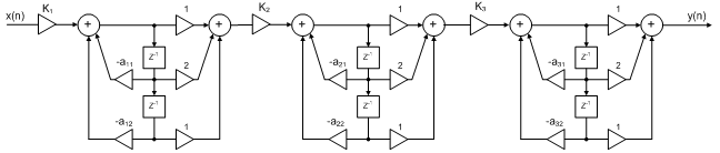
Figure 2. 6th order lowpass filter using
three biquads
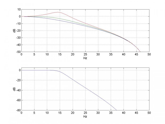
Figure 3. 6th order lowpass Butterworth cascaded-biquad response. fc= 15 Hz, fs= 100 Hz.
Top: response of each biquad section (blue= h1, green= h2, red= h3).
Bottom: overall response
Coefficient Quantization
As I stated at the beginning, the cascaded-biquad design is less sensitive to coefficient quantization than a single high-order IIR, particularly for lower cut-off frequencies. To illustrate this, we’ll first look at how quantizing coefficients effects z-plane pole locations of a 6th order IIR filter. The following code finds the unquantized poles of the 6th order Butterworth filter with -3 dB frequency fc = 5 Hz. (Note butter [6] is a function in the Matlab signal processing toolbox that synthesizes IIR Butterworth filters).
    fc= 5;
    fs= 100;
    [b,a]= butter(6,2*fc/fs);     % Matlab function for Butterworth LP IIR
    p= roots(a);                  % poles in z-plane
The poles are plotted as the red x’s on the left side of Figure 4. We have also plotted the poles for fc= 12 Hz (blue-ish x’s). Each set contains 6 poles. If we plot the poles of filters having fc from 1 Hz to 25 Hz in 1 Hz increments, we get the plot on the right, where only the right side of the unit circle is shown. The lower values of fc are on the right, near z = 1.
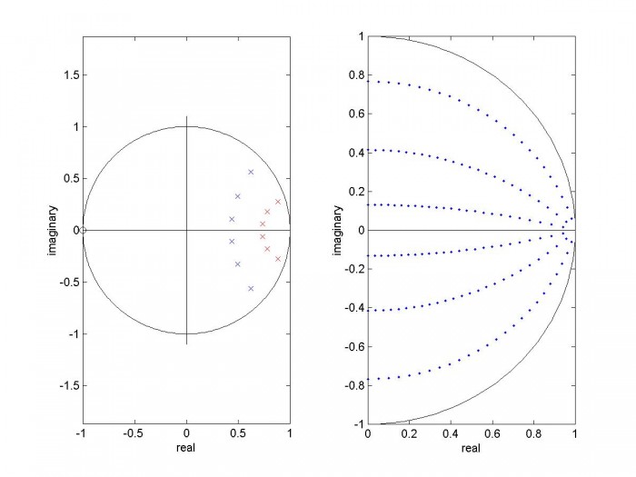
Figure 4. Unquantized poles of 6th-order Butterworth IIR filter.
Left: fc = 5 Hz (red) and 12 Hz (blue). Right: fc = 1 Hz to 25 Hz.
Now let’s quantize the denominator coefficients and see how this effects the pole locations of Figure 4. Let nbits = the number of bits per unit of coefficient amplitude:
nbits= 16;
Here is the code to find the quantized poles for a single value of fc:
    fs= 100;
    [b,a]= butter(6,2*fc/fs);
    a_quant= round(a*2^nbits)/2^nbits;
    p_quant = roots(a_quant);
Letting fc vary in 0.5 Hz increments from 0.5 to 25 Hz, we get the poles shown on the left of Figure 5. As you can see, as fc decreases, quantization causes the poles to depart from the desired locations. The right side of Figure 5 shows the effect of 10-bit quantization.
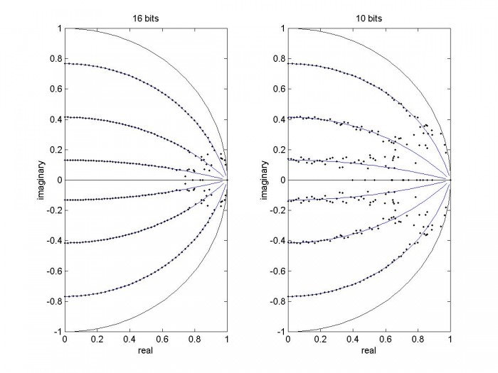
Figure 5. Effect of Quantization on poles of 6th-order Butterworth IIR filter.
Left: nbits = 16 Right: nbits = 10
We can do the same calculation for the biquads that make up the 6th order cascaded implementation. For example, here is the code to find the quantized poles of the second biquad for a single value of fc (recall that the matrix a has three rows containing the coefficients of 3 biquads).
    nbits= 10;
    a= biquad_synth(6,fc,fs);
    a2= a(2,:);                   % 2nd biquad
    a_quant= round(a2*2^nbits)/2^nbits;
    p_quant = roots(a_quant);
This time, letting fc vary in 0.25 Hz increments
from 0.25 to 25 Hz, we get the poles shown in Figure 6, which includes only
quadrant 1 of the unit circle. The
biquad performs much better than the 6
th order filter, only
departing dramatically from the unquantized curve for fc = 0.25 Hz. So we expect better performance from
cascading three biquads vs. using a single 6
th-order filter.
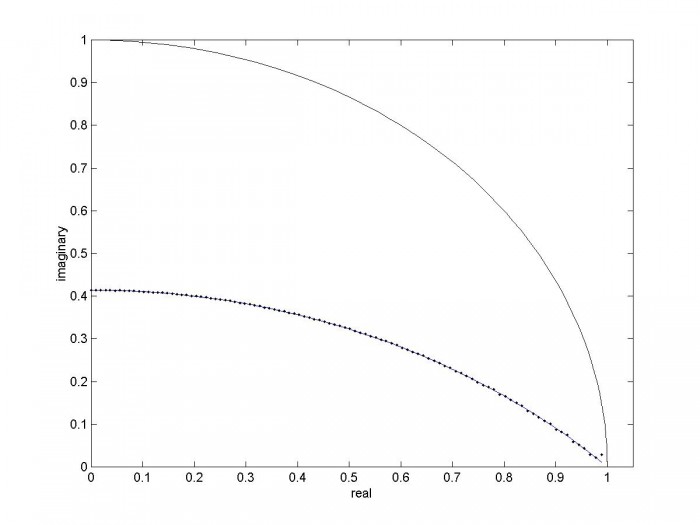
Figure 6. Effect
of Quantization on poles of one biquad, nbits = 10.
Now we’re finally ready to compare frequency response of a biquad-cascade filter vs. a conventional IIR filter when the denominator coefficients are quantized. The cutoff frequency and quantization level are chosen to stress the conventional filter. We’ll leave the numerator coefficients of the conventional filter as floating-point. Interestingly, when implementing the biquad filter we get exact numerator coefficient values “for free”: since b = [1 2 1], we can implement b0 and b2 as no-ops and b1 as a bit shift.
For the biquad filter, we use biquad_synth to find the coefficients for fc = 6.7 Hz:
    fc=6.7;     % Hz  -3 dB frequency
    fs= 100;    % Hz  sample frequency
    a = biquad_synth(6,fc,fs)  % a has 3 rows, one for each biquad
    a =
        1.0000   -1.3088    0.4340
        1.0000   -1.4162    0.5516
        1.0000   -1.6508    0.8087
For the conventional filter, we again use the Matlab function butter:
    [b,a]= butter(6,2*fc/fs);
    a = 1.0000   -4.3757    8.1461   -8.2269    4.7417   -1.4761    0.1936
In each case, we quantize coefficients to 10 bits per unit of coefficient amplitude:
    nbits= 10;
    a_quant= round(a*2^nbits)/2^nbits;           % quantize denom coeffs
First, we’ll look at the quantized pole locations. For the conventional filter, the quantized poles are:
p_quant= roots(a_quant);
For the biquad implementation, the quantized poles are:
    p1= roots(a_quant(1,:))’;
    p2= roots(a_quant(2,:)’;
    p3= roots(a_quant(3,:)’;
    p_quant= [p1 p2 p3];
Figure 7 shows the z-plane poles for the floating-point and quantized coefficients. Quantization has little effect on the biquad version, but has a large effect on the conventional filter.
Now let’s compare the magnitude responses for quantized coefficients. We compute the response of the biquad version in the same way used to obtain Figure 3. Figure 8 shows the magnitude responses. As you would expect from the pole plots, the conventional implementation has poor performance, while the biquad implementation shows no noticeable effect due to quantization.
So how low can we go with this N= 6 Butterworth cascaded-biquad filter? As we reduce fc, the quantization of 1024 steps per unit of coefficient amplitude eventually takes a toll. Figure 9 shows the z-plane poles and magnitude response for fc= 1.6 Hz. As you can see, the magnitude response is sagging. If we stay above fc of 2.5 Hz = fs/40, the response error is less than 0.1 dB.
Besides adding coefficient bits, there are other ways to improve performance of narrow-band IIR filters. See for example the post in reference [7].
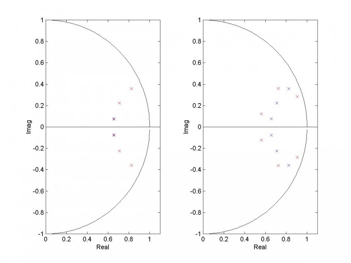
Figure 7. Z-plane pole locations with quantized denom. coeffs. N= 6, fc= 6.7 Hz, fs= 100 Hz.
Blue = floating point, Red = 10 bit quantization.
Left: biquad implementation Right: conventional implementation.
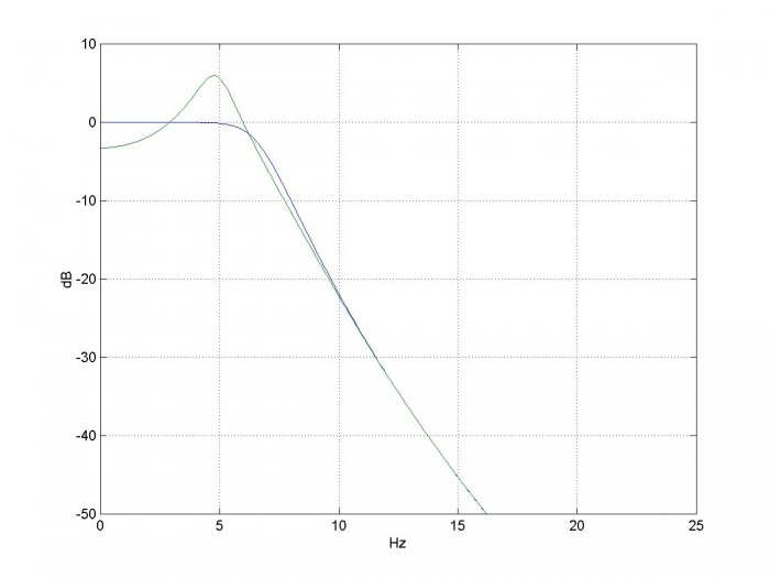
Figure 8. Magnitude response with quantized denom coeffs. N= 6, fc= 6.7 Hz, fs= 100 Hz, nbits = 10.
Blue = biquad implementation, green= conventional implementation.
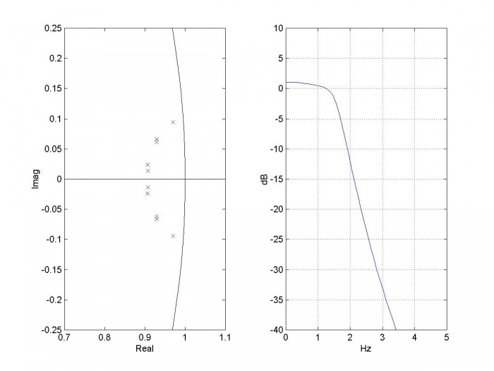
Figure 9. Z-plane poles and magnitude response of biquad-cascade filter with quantized denominator coefficients. Blue x’s = floating-point and red x’s = quantized. N= 6, fc= 1.6 Hz, fs= 100 Hz, nbits= 10.
References
1. Oppenheim, Alan V. and Shafer, Ronald W., Discrete-Time Signal Processing, Prentice Hall, 1989, sections 6.3.2 and 6.8.1.
2. Lyons, Richard G., Understanding Digital Signal Processing, 2nd Ed., Pearson, 2004, section 6.8.2
3. Robertson, Neil , “Design IIR Butterworth Filters Using 12 Lines of Code”, Dec 2017 https://www.dsprelated.com/showarticle/1119.php
4. Sanjit K. Mitra, Digital Signal Processing, 2nd Ed., McGraw-Hill, 2001, section 6.4.1
5. “Digital Biquad Filter”, https://en.wikipedia.org/wiki/Digital_biquad_filter
6. Mathworks website, ”butter”, https://www.mathworks.com/help/signal/ref/butter.html
7. Lyons, Rick, “Improved Narrowband Lowpass IIR Filters”, https://www.dsprelated.com/showarticle/120.php
Neil Robertson February 11, 2018 revised 2/20/18, 4/18/19
Appendix Matlab Function biquad_synth
This program is provided as-is without any guarantees or warranty. The author is not responsible for any damage or losses of any kind caused by the use or misuse of the program.
% biquad_synth.m    2/10/18 Neil Robertson
% Synthesize even-order IIR Butterworth lowpass filter as cascaded biquads.
% This function computes the denominator coefficients a of the biquads.
% N= filter order (must be even)
% fc= -3 dB frequency in Hz
% fs= sample frequency in Hz
% a = matrix of denominator coefficients of biquads.  Size = (N/2,3)
%     each row of a contains the denominator coeffs of a biquad.
%     There are N/2 rows.
% Note numerator coeffs of each biquad= K*[1 2 1], where K = (1 + a1 + a2)/4.
%
function a = biquad_synth(N,fc,fs);
if fc>=fs/2;
  error('fc must be less than fs/2')
end
if mod(N,2)~=0
    error('N must be even')
end
%I.  Find analog filter poles above the real axis (half of total poles)
k= 1:N/2;
theta= (2*k -1)*pi/(2*N);
pa= -sin(theta) + j*cos(theta);     % poles of filter with cutoff = 1 rad/s
pa= fliplr(pa);                  %reverse sequence of poles – put high Q last
% II.  scale poles in frequency
Fc= fs/pi * tan(pi*fc/fs);          % continuous pre-warped frequency
pa= pa*2*pi*Fc;                     % scale poles by 2*pi*Fc
% III.  Find coeffs of biquads
% poles in the z plane
p= (1 + pa/(2*fs))./(1 - pa/(2*fs));      % poles by bilinear transform
% denominator coeffs
for k= 1:N/2;
    a1= -2*real(p(k));
    a2= abs(p(k))^2;
    a(k,:)= [1 a1 a2];             %coeffs of biquad k
end
..
- Comments
- Write a Comment Select to add a comment
Wow. This a great article, Sir. Thank you.

You are welcome!
Thanks Neil! This was very helpful!
Here's a Python port of your biquad_synth function:
import numpy as np

def biquad_synth(N, fc, fs):

    fc = np.float64(fc)
    fs = np.float64(fs)

    if fc >= fs/2:
        raise Exception('fc must be less than fs/2')

    if N % 2 != 0:
        raise Exception('N must be even')

    # I. Find analog filter poles above the real axis (half of total poles)
    k = np.arange(N/2) + 1.0
    theta = (2 * k - 1) * np.pi / (2 * N)
    pa = -np.sin(theta) + 1j * np.cos(theta) # poles of filter with cutoff = 1 rad/s
    pa = np.flipud(pa) # reverse sequence of poles - put high Q last

    # II. scale poles in frequency
    Fc = fs/np.pi * np.tan(np.pi * fc / fs)
    pa = pa * 2 * np.pi * Fc # scale poles by 2*pi*Fc

    # III. Find coeffs of digital filter
    # poles and zeros in the z plane
    p = (1 + pa / (2 * fs)) / (1 - pa / (2 * fs)) # poles by bilinear transform

    # denominator coeffs
    return np.stack((np.ones(N/2), -2 * np.real(p), np.abs(p)**2)).transpose()
Hi 5plic3r,
Thanks for the code.
Neil
Could a similar technique be used for a high-pass Butterworth?
Yes, I think the technique is general.
Neil
Based on your Design IIR Highpass Filters article, I tried to get a high-pass version by changing this
pa = pa * 2 * np.pi * Fc
to this
pa = 2 * np.pi * Fc / pa
But I'm see the same results. Am I heading in the right direction?
Thanks!
The LP to HP transformation of the poles is:
pa= 2*pi*Fc./p_lp;
Then the change to the numerator coeffs and scaling is:
b= [1 -2 1]; % hp biquad numerator coeffs
for i= 1:N/2;
K(i)= sum(a(i,1)- a(i,2)+ a(i,3))/4;
end
Dear Mr. Robertson,
thanks a lot for all the great articles - they are really helpful and I appreciate them!
I was just wondering about a comment in your code: "put high Q last".
Why is this?
Is there some general advice on how to order biquad stages (regarding any filter, i.e. lp, hp or bp) - I guessed the gain would be the most interesting figure to look at - but maybe I am wrong and it is indeed Q.
Any explanations on this topic would be greatly appreciated.
Sincerely,
Daniel
Hi Daniel,
Here is a quote from the post's text on that topic:
"The magnitude response of each biquad and the overall response are plotted in Figure 3. The sequence of the biquads doesn’t matter in theory; however, placing the biquad with the peaking response (h3) last minimizes the chance of clipping."
If you look at figure 3, the h3 section has max gain greater than 1.0 near 14 Hz. So if you had a signal near that frequency with level near 1.0, you would have clipping or rollover in that section (assuming a max signal range of +/-1). The h1 and h2 sections have loss at 14 Hz. So if you place them before the h3 section, it will make clipping less likely.
If you look at the poles of the overall filter, the h3 section's poles are closest to the unit circle ("highest Q"). So it makes sense to order the sections of a LPF according to their distance from the unit circle: farthest first to closest last.
For a few words on ordering/scaling of the sections of a cascaded-biquad BPF, see my post https://www.dsprelated.com/showarticle/1257.php
regards,
Neil
Hello Neil,
thanks for your reply. Me (and me colleague) still are interested to understand the whole story.
I was stumbling about your quotes ^^:
("highest Q")
... and I guess your advice is a pragmatic approach towards using the center of the z-plane / the absolute value of the poles as a measure for sorting the poles when using cascaded biquads.
I found a nice plot on Stackexchange that illustrates equipotential levels of Q in the z-plane: https://dsp.stackexchange.com/questions/19148/whats-the-q-factor-of-a-digital-filters-pole
They tend to be similar, but not exactly the same thing as the distance to the center / the unit sphere bound. I guess the difference is most crucial when we are dealing with very narrow banded filters at lower frequencies (relative to the sampling rate) - which is, unfortunately, exactly what we are heading for at the moment.
So, the "by-the-bool" solution would be to use Q indeed and not |z|, or is there still something I am missing?
Sincerely,
Daniel
Daniel,
Maybe there is no need to bring the concept of Q into the discussion. Maybe it's simpler to just say that the biquad sections are ordered starting with the pole-pairs closest to the unit circle.
For a Butterworth LPF, the poles fall on a nice circle in the z-plane, so there should not normally be any ambiguity about ordering.
Of course, it is not required to use any particular ordering if you allow extra headroom in your adders to account for the biquad gain exceeding 1 over a portion of the frequency range.
Finally, I don't claim to be an expert on IIR filter design -- I'm just trying to illustrate some basics!
regards,
Neil
Very good article.
Clarify my DSP concept.
Thanks for the encouragement!
Neil
I have a question about design Bessel filter.
To find the pole of Bessel filter, the frequency normalization process required the division of Thomson’s values by a factor(Bessel Normalizing Factors), as follows:
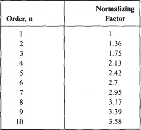
But I using these factor to calculate the pole of the Bessel filter, the pole are not same as MATLAB besselap.m, as follows:
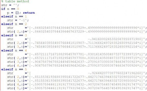
This problem has troubled me for a long time.
Herbert
Herbert,
Sorry, I don't know the answer to your question.
Neil
Neil,
You are welcome.
Herbert

Herbert,
this question belongs in the forum I think - feel free to ask it there.
OK, thanks.
Herbert
Thank you sir. Realy good article. I want to as a question with your permission.
MATLAB always setting b=[1,2,1]. But when I search different web sites, this matrix can changable. What's the reason of this situation.
I want to implement this filter in my embedded project via C code. How can i implement this filter.
Thank you and have a nice day.
Hi,
I'm not sure I understand your question. In my article, each biquad has 2 zeros at z = -1, so the numerator of each biquad is (z + 1)(z + 1) = z^2 + 2z + 1, or equivalently 1 + 2z^-1 + z^-2. Thus each biquad has b = [1 2 1]. As I discussed, these are the zeros resulting from the bilinear transform of the analog lowpass zeros.
This choice of zeroes means that the frequency response has a null at fs/2, which is a sensible choice for lowpass filters.
regards,
Neil
Hello Sir,
thank you so much for your great article.I would like to follow your example.
Can you provide me your matlab code to plot Figure 3?
Hi,
Here is the code.
% biquad_ex1.m     2/7/18 nr
%  Plot overall response and responses of biquads for N= 6 Butterworth
% a = matrix of denominator coeffs  size = N/2 by 3
% a(1,:) = first biquad
% a(2,:) = 2nd biquad
% a(N/2,:) = last biquad
N= 6;              % note N is not programmable in this m-file
fc= 15;
fs= 100;
%  Synthesize filter using N/2 biquads
a = biquad_synth(N,fc,fs)
b= [1 2 1];        % biquad numerator coeffs
for i= 1:N/2;
   K(i)= sum(a(i,:))/4;
end
K
% find frequency response
[h1,f]= freqz(K(1)*b,a(1,:),512,fs);
[h2,f] = freqz(K(2)*b,a(2,:),512,fs);
[h3,f] = freqz(K(3)*b,a(3,:),512,fs);

h= abs(h1.*h2.*h3);
H= 20*log10(abs(h));
H1= 20*log10(abs(h1));
H2= 20*log10(abs(h2));
H3= 20*log10(abs(h3));
%
%plotting
subplot(211),plot(f,H1,f,H2,f,H3),grid
axis([0 fs/2 -50 10])
xlabel('Hz'),ylabel('dB')
subplot(212),plot(f,H),grid
axis([0 fs/2 -80 5])
xlabel('Hz'),ylabel('dB')
Thanks for sharing the matlab code.
If I use the filter designer to design a Butterworth LP 6th order with the same frequencies. Are the coefficients completely different. Why is that ?
Sorry, I don't understand your question. What do you mean by "the filter designer". You say the coefficients are "completely different". Completely different from what?
I mean the the "app" from matlab the "filter designer" from the dsp toolbox.
So sorry. I use the wrong fc from you example in the filter designer.
But my next question is.
Could i use fs=1.0 and fc=0.25?
to make a lowpass halfband butterworth filter?
i got the coefficients:
a =
    1.0000   -0.0000    0.0173
    1.0000   -0.0000    0.1716
    1.0000   -0.0000    0.5888

K =
    0.2543    0.2929    0.3972
You can certainly do that. As you can see, the a1 coeffs are always zero.
Note that the term halfband is normally used to describe an FIR filter. Halfband FIR filters have fc = fs/4 and every other tap value is zero (except for the main tap). FIR filters have the advantage that the phase response is linear, while IIR filter's phase response is not linear.
To post reply to a comment, click on the 'reply' button attached to each comment. To post a new comment (not a reply to a comment) check out the 'Write a Comment' tab at the top of the comments.
Please login (on the right) if you already have an account on this platform.
Otherwise, please use this form to register (free) an join one of the largest online community for Electrical/Embedded/DSP/FPGA/ML engineers: