Interpolation Basics

This article covers interpolation basics, and provides a numerical example of interpolation of a time signal.  Figure 1 illustrates what we mean by interpolation.  The top plot shows a continuous time signal, and the middle plot shows a sampled version with sample time T_s.  The goal of interpolation is to increase the sample rate such that the new (interpolated) sample values are close to the values of the continuous signal at the sample times [1].  For example, if we increase the sample rate by the integer factor of four, the interpolated signal is as shown in the bottom plot.  The time between samples has been decreased from T_s to T_s/4.

The simplest technique for interpolation is linear interpolation, in which you draw a straight line between sample points, and compute the new samples that fall on the line.  However, in many cases, linear interpolation is not accurate enough.  Other techniques involve fitting polynomials to the time function.  Here, we’ll show the power of approaching the problem in the frequency domain.

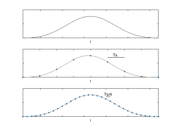
Figure 1.  Top:  Continuous signal       

Middle:  Signal with sample time T_s  

Bottom:  Interpolated signal with sample time T_s/4  

Before we describe how interpolation works, let’s look at two sampled signals and their spectra.  In the top row of Figure 2, the time signal u is sampled at 400 Hz, and its magnitude spectrum is shown on the right.  In the bottom row, the time signal x consists of every fourth sample of u, and thus has sample rate of 100 Hz.  The spectrum is again shown on the right, with the image spectrum above 100 Hz shown by a dashed line.  Note the amplitude of the spectrum is ¼ that that of u.

Now let’s look at an example of interpolation by an integer factor of four.  For the signal x just described, interpolation by four should result in the signal u.  Matlab code for the example interpolator is provided at the end of the article.

If we simply increase the sample rate of x from 100 Hz to 400 Hz, we get the signal shown in Figure 3.  Here we’ve just inserted three zeros between each of the original samples of x, a process called upsampling.  Upsampling includes scaling the amplitude of x by the upsampling ratio of 4, which gives a maximum spectrum magnitude of 1, instead of 1/4.  The spectrum of the upsampled signal x_up is shown on the right.  Given that x_up sample values have the same time spacing as x, the spectrum is the same as that as x, except its amplitude is a factor of 4 larger.

Now, if we compare the spectrum of x_up to that of u, they match from 0 to 50 Hz, but x_up has additional image spectra centered at 100 and 200 Hz.  So, it seems that we should be able to approximate u by low-pass filtering x_up to attenuate the images.  If this works, we will have interpolated x by four.  A block diagram of the interpolator is shown in Figure 4.  In our case L = 4.

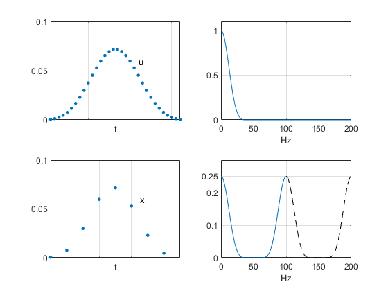
Figure 2.  Top:  sampled signal u with f_s = 400 Hz and its spectrum (linear amplitude scale)

Bottom:   sampled signal x with f_s = 100 Hz and its spectrum

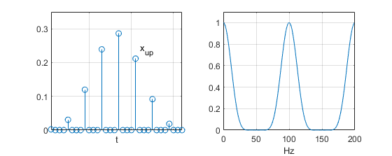
Figure 3.  Upsampled signal x_up with f_s = 400 Hz and its spectrum (linear amplitude scale)

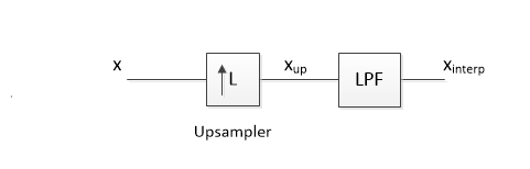
Figure 4.  Interpolator block diagram (for our example, L = 4)             

To design the low-pass filter, we’ll look at the dB spectrum of x_up, as shown in the top of Figure 5.  We need a filter that passes the desired spectrum and attenuates the undesired images.  Thus, we have the following passband and stopband:

Passband:  0 to 36 Hz

Stopband:  66 to 135 Hz and 166 to 200 Hz

We leave the ranges from 50 to 66 Hz and 135 to 166 Hz unspecified, since the amplitude of x_up’s spectrum is low in these ranges.  The Matlab code at the end of this article includes synthesis of a 41-tap FIR interpolation filter.  The filter response is shown in the middle of Figure 5.  The spectrum of x_interp is shown in the bottom plot.

The time signal x_interp is shown on the left of Figure 6, with the linear-amplitude spectrum on the right.  As hoped, x_interp resembles the plot of u in Figure 2.   We can compute the error between x_interp and u as:

% error = 100*(x_interp – u)/max(u)

The error is plotted in Figure 7.   Reflecting on how we achieved this result, it is worth noting that we performed interpolation in time by applying knowledge of the input signal’s frequency spectrum.

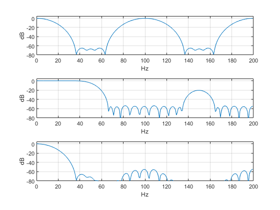
Figure 5.  Top:  Spectrum of x_up            

Middle:  Interpolation low-pass filter response          

Bottom:  Spectrum of x_interp          

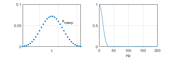
Figure 6.  Left:  Interpolator output x_interp (compare to u in Figure 2)

Right:  spectrum of x_interp (linear amplitude scale)

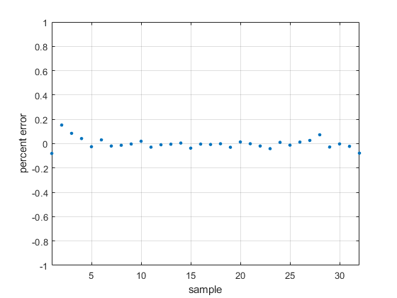
Figure 7.  Interpolation percent error                 

Matlab code demonstrating interpolation by four

The following code uses the same signal names as the text:

u                        signal sampled at 400 Hz

x                        interpolator input signal (formed from every 4^th sample of u)

x_up                  upsampled version of x, f_s = 400 Hz

x_interp             interpolation filter output, f_s = 400 Hz

The signal u is a Chebyshev window function of length 32 with -70 dB sidelobes [2,3].  Other functions could be used, for example a Blackman window.  As previously discussed, the calculation of x_up includes scaling by 4.  The interpolator output x_interp has length 72.  Samples 21:52 are used as an approximation of the signal u.

The interpolation filter has fs = 400 Hz and is synthesized using the Parks-McClellan algorithm (Matlab function firpm).  The coefficients are plotted in Figure 8, and the filter’s frequency response is shown in the center plot of Figure 5.  Note that while this design approach is straightforward, it does not result in the most efficient interpolator.  One alternative approach would cascade two interpolate-by-two sections, as shown in Figure 9.  This allows the use of halfband interpolation filters [4].  For a discussion of efficient approaches to interpolator design, see [5].

%interp_demo.m  8/17/2019 Neil Robertson
% Demonstrate interpolation by 4
fs= 400;                % Hz sample rate
p= chebwin(32,70)';     % signal = Chebyshev window
u= p/sum(p);            % normalize for sum = 1
x= [u(1:4:end)];        % interpolator input signal, fs= 100
% upsampling
x_up= zeros(1,32);
x_up(1:4:32)= 4*x(1:8); % upsampled signal
%
% interpolation filter using Parks-McClellan algorithm
fn= fs/2;
f= [0 36 66 135 166 199]/fn;    % frequency vector
a= [1 1 0 0 0 0];               % amplitude goal vector
Ntaps= 41;
b= firpm(Ntaps-1,f,a);          % synthesize filter coeffs
b= round(b*2^13)/2^13;          % fixed point coeffs
%
x_interp= conv(x_up,b);         % filter x_up
interp_error= 100*(x_interp(21:52) - u)/max(u);
%
[Xup,f]= freqz(x_up,1,256,fs);      % spectrum of x_up
Xinterp= freqz(x_interp,1,256,fs);  % spectrum of x_interp
%
%
% plotting
subplot(211),plot(u,'.','markersize',10),grid
axis([1 32 0 .1]),xticklabels({}),text(23,.06,'u')
subplot(212),plot(x,'.','markersize',10),grid
axis([1 9 0 .1]),xticklabels({}),text(6.5,.06,'x'),figure
stem(b),grid
axis([1 41 -.05 .3]),title('Interpolation Filter Coefficients b')
figure
subplot(211),stem(x_up),grid
axis([1 32 0 .35]),xticklabels({}),text(23,.24,'x_{up}')
subplot(212),plot(x_interp(21:52),'.','markersize',10),grid
axis([1 32 0 .1]),xticklabels({}),text(23,.06,'x_{interp}'),figure
plot(interp_error,'.','markersize',10),grid
axis([1 32 -1 1]),xlabel('sample'),ylabel('percent error')
title('Interpolation Percent Error'),figure
subplot(211),plot(f,abs(Xup)),grid
xlabel('Hz')
axis([0 fs/2 0 1]),title('Spectrum of x_{up} (linear amplitude scale)')
subplot(212),plot(f,abs(Xinterp)),grid
xlabel('Hz')
axis([0 fs/2 0 1]),title('Spectrum of x_{interp} (linear amplitude scale)')

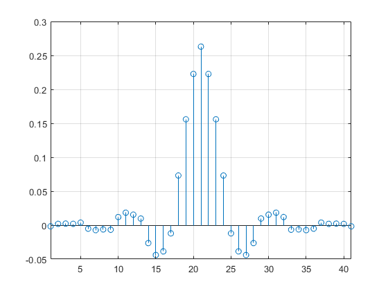
Figure 8.  Interpolate-by-four filter coefficients.     

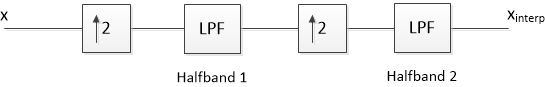
Figure 9.  Interpolation by four using two Interpolate-by-two stages.

References

1. Lyons, Richard G., Understanding Digital Signal Processing, 3^rd Ed., Prentice-Hall, 2011, section 10.4.
2. The Mathworks website, https://www.mathworks.com/help/signal/ref/chebwin.html
3. Wikipedia, “Window Function”, https://en.wikipedia.org/wiki/Window_function
4. Robertson, Neil, “Simplest Calculation of Halfband Filter Coefficients”, https://www.dsprelated.com/showarticle/1113.php
5. Harris, Fredric J., Multirate Signal Processing for Communication Systems, Prentice Hall, 2004, Ch 7.

Neil Robertson               August, 2019

Sign in