Lost Secrets of the H-Bridge, Part III: Practical Issues of Inductor and Capacitor Ripple Current
We've been analyzing the ripple current in an H-bridge, both in an inductive load and the DC link capacitor. Here's a really quick recap; if you want to get into more details, go back and read part I and part II until you've got equations coming out of your ears. I promise there will be a lot less grungy math in this post. So let's get most of it out of the way:

Switches QAH and QAL are being turned on and off with pulse-width modulation (PWM), to produce an average voltage DaVdc on one side of the load, while switches QBH and QBL are being turned on and off to produce an average voltage DbVdc on the other side. The average voltage across the load is \( (D_a - D_b) V _ {dc} = DV _ {dc} \).
The load current \( I_L \) consists of a DC and low-frequency current \( I_{Ldc} \), which we want, combined with a sawtooth-like AC ripple component that contains harmonics of the switching frequency, which we're stuck with. (Actually this isn't true in all switching converter topologies; some use coupled inductors to cancel out ripple current in the input or output of the circuit.)
We can coordinate the switching waveforms of the two phases of the H-bridge, so that they are edge-aligned or center-aligned PWM. In general, center-aligned is the best choice, and in an H-bridge if we use center-aligned PWM with \( D_a \) and \( D_b \) such that \( D_0 = \frac{D_a + D_b}{2} = \frac{1}{2} \), then this minimizes the magnitude of ripple current, and gets rid of odd harmonics of the switching frequency, so that the effective ripple frequency is twice the ripple frequency found at edge-aligned PWM.
For edge-aligned PWM, and for center-aligned PWM with D0 = 0.5, the ripple current in the load is a simple triangle wave; otherwise the ripple current is a double-toothed triangle wave.
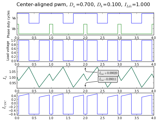
Generally the DC link is designed with capacitors to shoulder the burden of high-frequency current drawn from the DC link, so that the voltage source sees only DC and low-frequency current \( I_S \). The DC link capacitor current \( I_{CDC} \) has an average value of zero, and can be analyzed easily by knowing the two duty cycles \( D_a \) and \( D_b \) and the DC load current \( I_{Ldc} \).
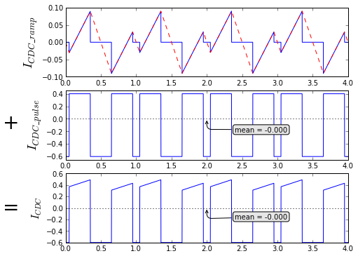
The DC link capacitor current can be decomposed into two parts: ramp current, which is a small sawtooth-like ripple that results from the load current ripple and is independent of DC load current; and pulse current, which is a square-wave-like ripple that results from the load current being switched on and off of the DC link. These components both have an average value of zero, and are orthogonal, so that their RMS values can be calculated and combined to identify the total RMS capacitor current.
If you crunch the numbers, here's some quantitative statistics you can come up with to describe the inductor and capacitor currents:
\( D = D_a - D_b \) is the effective load duty cycle
\( D_0 = (D_a + D_b)/2 \) is the common-mode duty cycle
\( I_{CDC} \) is the current flowing out of the DC link capacitor
\( I_S = DI_{Ldc} \) is the supply current
\( I_{R0} = V_{DC}T/L \) is a reference current that simplifies calculation of these statistics.
\( I_R = |D|(1-|D|)I_{R0} \) is a differential duty-cycle dependent ripple current
\( I_{R2} = 2|D||D_0-\tfrac{1}{2}|I_{R0} \) is a common-mode duty-cycle dependent ripple current
\( I_{Lpk} \) = Mean-to-peak load current ripple. (Since the load current ripple is symmetric, the peak-to-peak load current is \( 2I_{Lpk} \).)
\( I_{Lrms} \) = RMS load current ripple (does not include DC)
| PWM type | \( I_{Lpk} \) | \( I_{Lrms} \) | fundamental frequency | amplitude of kth harmonic of load current |
|---|---|---|---|---|
| edge-aligned | \( \tfrac{1}{2}I_R \) | \( \frac{1}{2\sqrt{3}}I_R \) | \( f_{PWM} = 1/T \) | $$A_k = \frac{(-1)^k \sin k\pi D}{k^2\pi^2} I_{R0}$$ |
| center-aligned (common-mode = 0.5) |
\( \tfrac{1}{4}I_R \) | \( \frac{1}{4\sqrt{3}}I_R \) | \( 2f_{PWM} \) | $$A_k = \frac{(-1)^k \sin k\pi D}{2k^2\pi^2} I_{R0}$$ |
| center-aligned (common-mode ≠ 0.5) |
\( \tfrac{I_R+I_{R2}}{4} \) | \( \frac{|D|\sqrt{12(D_0-\tfrac{1}{2})^2 + (1-|D|)^2}}{4\sqrt{3}}I_{R0} \) | \( {f_{PWM}}^ * \) | exercise for the reader |
*1st harmonic of capacitor current in center-aligned PWM has low amplitude if D0 is close to 0.5
These statistics about DC link capacitor current can be expressed independent of the PWM type:
| statistic | symbol | value | conditions |
|---|---|---|---|
| peak-to-peak | \( I_{CDCpkpk} \) | \( |I_{Ldc}| + I_{Lpk} \) | |
| positive peak | \( I_{CDCpeak+} \) | \( |I_{Ldc}|(1-|D|) + I_{Lpk} \) | \( I_S > 0 \) (positive power) |
| negative peak | \( I_{CDCpeak-} \) | \( -I_S \) | |
| positive peak | \( I_{CDCpeak+} \) | \( -I_S \) | \( I_S < 0 \) (regeneration) |
| negative peak | \( I_{CDCpeak-} \) | \( -|I_{Ldc}|(1-|D|) - I_{Lpk} \) | |
| RMS | \( I_{CDCrms} \) | \( \sqrt{|D|}\sqrt{{I_{Lrms}}^2 + (1-|D|)I_{Ldc}^2} \) | |
| amplitude of kth harmonic |
\( A_k \) | $$\underbrace{\frac{j(1-|D|) I _ {R0} (\sin k\pi |D| - k\pi |D| \cos k\pi |D|)}{mk^2\pi ^2}} _ {\text{ramp current} ^ *} + \underbrace{\frac{2I _ {Ldc} \sin k\pi D}{k\pi}} _ {\text{pulse current}}$$ |
* \( m=1 \) for edge-aligned PWM, \( m=2 \) for center-aligned PWM with \( D_0 = \tfrac{1}{2} \). Calculating \( A_k \) for the general case of center-aligned PWM (\( D_0 \neq \tfrac{1}{2} \)) is an exercise for the reader.
What do inductors and capacitors care about all this?
While I don't really mind if you don't care about all this math, I do mind what the inductor and capacitor care about it.
Note that load inductance and DC link capacitance are good things, in general; they keep the load current steady and the DC link voltage steady. So we have to keep our components happy!
Ripple current in the load
There are a few reasons why load current ripple is of concern:
- The extra RMS current uses up design margin for thermal rise in the load.
- The extra peak current uses up design margin for inductor saturation and overcurrent sensing.
- The switching frequency harmonics can cause electromagnetic interference (EMI).
Remember that the only current we really want in the load is the DC and low-frequency components. When you buy a component with inductance, like an inductor or a motor or a transformer, you are paying for current-handling capability, and if you've done a good job in your system design, that capability will be used but not overused.
RMS current
Let's say that I have a system where I need to support load currents with low-frequency content containing 9.5A at DC combined with a 4.5A sine wave at 500Hz. This has an RMS value of just over 10A, and a peak value of 14A.
import matplotlib.pyplot as plt
import numpy as np

tmax = 4e-3
dt = 0.5e-6
t = np.arange(0,tmax,dt)
t_msec = t/1e-3
I_Ldc0 = 9.5
f = 500
I_Ldc = I_Ldc0 + 4.5*sin(2*np.pi*f*t)
plt.plot(t_msec,I_Ldc,[0,tmax/1e-3],[I_Ldc0]*2,':k')
plt.ylim(0,14.5)
plt.xlabel('time (msec)')

def rms(x):
    return np.sqrt(np.mean(x**2))
print "RMS(I_Ldc) = %.3fA" % rms(I_Ldc)
RMS(I_Ldc) = 10.019A

When conductive losses in the load are a limiting factor, for the most part this corresponds to RMS load current.
Let's say I'm working with a Magnetics Guy (he's the one who pulls out Col. McLyman's book and does all sorts of black art calculations to design inductors and transformers and whatnot) who tells me that we have just enough design margin to pull off 10A RMS load current, if we needed more then he'd have to go to a bigger core size and they don't have any in stock right now, so he's glad we only need the 10A RMS, and speaking of overheating, it's been one long hot summer, and hey, did you see the Red Sox game last night, after the third inning—
Then I tell him I'm working on this H-bridge, and I had to decrease the switching frequency to reduce switching losses, so we're going to have to account for more ripple current.
"How much ripple current?" he asks, with sudden fear in his eyes.
It might be an amp or two, we'll have to check what it looks like—
"I'll give you another 2% thermal rise," he says, frowning. "That's 10.1A RMS. No more than that."
Another 2% increase in I2R losses means a 1% increase in RMS current; we can go from 10Arms to 10.1Arms. Doesn't sound like much, does it?
The good news is that RMS adds in quadrature for uncorrelated waveforms: DC is uncorrelated with low-frequency zero-mean waveforms, so the RMS value of our 9.5Adc current plus 4.5A peak (=3.182Arms) low frequency current gives us an RMS magnitude of \( \sqrt{9.5^2 + 3.182^2} = 10.019 \)A. The major component of RMS is greatly dominated by its largest amplitude.
How much more can we add to this with high-frequency ripple current? \( \sqrt{9.5^2 + 3.182^2 + x^2} = 10.1 \). Solve for x and you get x = 1.28A. We can add 1.28Arms of ripple current without blowing our thermal budget. Let's be conservative and try to use 0.75A rms ripple, just to leave some margin; this puts the total RMS current at just under 10.05A.
How much ripple current is 0.75Arms? Well, our formulas above say that for center-aligned PWM with \( D_0 = \frac{1}{2} \), which has a triangular ripple current waveform, the peak ripple current is \( \sqrt{3} \) times as much as the RMS value, or 1.30A peak. Here's what the resulting load current waveform would look like:
def showripple(t,I_Ldc,I_Lripple_pk,T = 100e-6,
     centeralign=True, showripple_alone=False):
  ''' show ripple current:
t is time waveform
I_Ldc is DC/low frequency current
I_Lripple_pk is the peak of the switching frequency ripple
T is the period of the current ripple waveform
'''
  fripple = (2.0 if centeralign else 1.0) / T
  u = abs(((t*fripple - 0.25) % 1)*2-1)*2-1
  I_Lripple = I_Lripple_pk * u
  t_msec = t/1e-3

  if showripple_alone:
    plt.subplot(2,1,1)
    plt.plot(t_msec,I_Lripple)
    plt.ylabel('$I_{Lripple}$', fontsize=15)
    plt.subplot(2,1,2)

  I_L = I_Ldc + I_Lripple
  plt.plot(t_msec,I_L,t_msec,I_Ldc,'r')

  plt.ylim(min(0,np.amin(I_L)),np.amax(I_Ldc)+I_Lripple_pk*1.1)
  plt.ylabel('$I_L$', fontsize=15)
  plt.xlabel('time (msec)')
  print("RMS I_Ldc = %.3f, peak I_Ldc = %.3f" % (rms(I_Ldc),max(I_Ldc)))
  print("RMS I_L   = %.3f, peak I_L   = %.3f" % (rms(I_L),max(I_L)))

showripple(t,I_Ldc,1.3,T=100e-6,centeralign=True,
   showripple_alone=True)
RMS I_Ldc = 10.019, peak I_Ldc = 14.000
RMS I_L   = 10.047, peak I_L   = 15.297
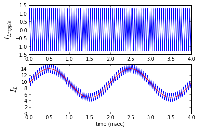
So I call the Magnetics Guy back over, after working through these numbers and tell him that we're looking at a worst-case scenario of 10.05A, only 1% thermal rise.
"What's the overall peak current?" he asks.
I know where this is going. I add up the numbers and tell him: 9.5Adc + 4.5A peak low-frequency sine wave + 1.30A peak switching ripple = 15.3A maximum.
He stares at you for a few seconds. "Look, I can give you 15A, that's it. More than that, and we won't have enough design margin for inductor saturation."
I tell him I can probably accommodate that: so I'm down to 1A peak switching ripple. After all, that's still pretty large: 2A peak-to-peak on a low-frequency waveform that's in the 5-14A range is pretty visible; take a look at the waveform below. But notice that the RMS ripple of the waveform as a whole barely budged.
showripple(t,I_Ldc,1.0,T=100e-6)
RMS I_Ldc = 10.019, peak I_Ldc = 14.000
RMS I_L   = 10.035, peak I_L   = 14.997
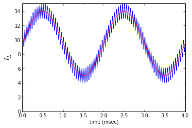
This is an important lesson: In order to make a significant increase to conduction (I2R) losses in the load, the switching ripple current has to be very large.
How large? Let's say we want to see how much ripple it takes to increase the RMS ripple by 5%, which increases the conductive losses by about 10%. That would put our total RMS current at 10.5A. Here's what that looks like:
showripple(t,I_Ldc,5.45,T=100e-6)
RMS I_Ldc = 10.019, peak I_Ldc = 14.000
RMS I_L   = 10.501, peak I_L   = 19.447
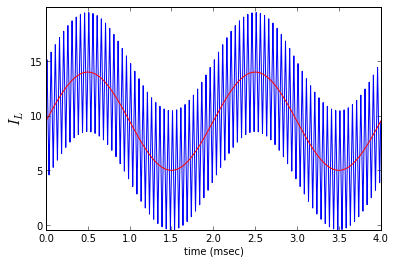
That's right: it takes just under 11A peak-to-peak ripple to bring us up to 10.5Arms. 11A peak-to-peak! That's huge! This waveform looks awful; we're actually getting negative load current for a brief instant. Anyone who's done power conversion would look at this and their stomach would turn in disgust. And yet we only get 10% more conduction losses.
You don't believe it? Try crunching the numbers yourself. I ran into this kind of situation a few years ago; we had more ripple current than we expected, and I was worried about extra conduction losses... until I crunched the numbers and realized the effect was minimal. So that's lesson #2: Crunch the numbers, and know what you're dealing with! If you know the impact of ripple current on your system, you can focus your efforts on things that are significant and not worry about the rest.
Speaking of crunching the numbers, let's put some more numbers into this example. We've been showing graphs based on T = 100μs, which corresponds to a switching frequency of 10kHz and a ripple current frequency of 20kHz with center-aligned PWM. Let's use Vdc = 24V, just because it's a nice round number often used in industrial automation systems. That just leaves L. What kind of inductance would give us a worst-case peak ripple of 1A we talked about earlier? Well, we do have an equation that says that for center-aligned PWM with \( D_0 = 0.5 \), the peak inductor switching ripple is \( \frac{1}{4}I_R = \frac{1}{4}|D|(1-|D|)I _ {R0} \); the maximum value of this is \( \frac{1}{16} I _ {R0} = \frac{V _ {dc}T}{16L} \) for \( D = \pm\frac{1}{2} \). Set to 1.0A and solve for inductance, and we get \( I _ {R0} = 16\text{A} \) and \( L = \frac{V _ {dc}T}{16\text{A}} = 150\mu H \). For an inductor this isn't a little surface-mount component; a 150 μH inductor rated at 15A peak and around 10A RMS is probably somewhere around the size of a golf ball or a 35mm film cartridge, maybe a little smaller, maybe a little larger — I found a few 100 μH 10A power inductors on Digikey and Mouser, and they were 2cm-3cm in length and roughly the same diameter.
Summary of example scenario
Remember these numbers for future reference. The scenario below is what we're going to use for some further analysis.
- Vdc = 24V
- Switching frequency = 10kHz, using center-aligned PWM, with Da = 0.75, Db = 0.25, D = 0.5
- Inductance = 150μH.
- Normalizing reference current \( I _ {R0} = \frac{V _ {dc} T}{L} = 16A \).
- Maximum load current = 9.5Adc + 4.5A peak low frequency sine wave + 1.0A peak switching ripple current.
- Maximum load current in terms of normalized reference current is \( 0.594 I _ {R0} \) DC + \( 0.281 I _ {R0} \) low frequency sine wave + \( 0.063 I _ {R0} \) switching ripple
- RMS load current = 10.035Arms at maximum load, including the effects of swtiching ripple current, vs. 10.019Arms without the effects of switching ripple current.
Peak current
So the good news is that the effect of switching ripple on total RMS current probably isn't a major concern. If you can find a load capable of carrying the current you want, it probably won't heat up much more from switching current ripple, unless the ripple waveform is awful. (But check it in each situation just to be sure!)
The bad news is that peak current is more likely to be a significant limit.
Let's do some thinking, and then run a little simulation. We'll take a hypothetical 150uH 15A peak inductor. Maximum rated current in an inductor is just an arbitrary threshold picked by the manufacturer. Usually it's specified as the point at which the manufacturer guarantees the inductance drops by a maximum of 5 or 10%. What happens is that at some point, the magnetic material starts to saturate. Air-core inductors are kind of lousy for achieving a desired amount of inductance in a given volume, and the magnetic field leaks all over the place. If you put ferrous metal or ferrites into a component, it can direct the magnetic field, keep it from leaking outside the component, and raise the inductance to a useable level. You change the current in an inductor, and below a certain limit, everything is nice and linear -- the current doubles, and so does the magnetic field. You put a constant voltage across the inductor for a certain amount of time, and the current ramps up linearly with time. The magnetic material helps keep that process slow. But magnetic materials also have a limited amount of magnetization they can reach; beyond that point, they look more and more like air and all of a sudden the current increases faster and faster. This is a gradual process, so it's not like if you have an inductor rated at 10A peak and you get to 10.5A the component will get immediately damaged and burst into flames. Instead its performance will be lower and you'll have higher losses. Let's try that simulation I talked about.
import math
def numderiv(f,eps):
    '''create a numerical derivative
using symmetrical differences'''
    def fprime(x):
        return (f(x+eps)-f(x-eps))/(eps*2)
    return fprime

def Lsat(L0, Irated, Lsag=0.1, k=8):
    ''' simulates a saturable inductor
using a sigmoid curve with adjustable sharpness k
y = x / (1 + x**k)**(1/k)
Inductance drops by Lsag at Irated
'''
    rho = ((1/(1.0-Lsag)) ** (k/(k+1.0)) - 1) ** (1.0/k)
    psi0 = L0*Irated/rho
    def fL(I):
       ''' flux = fL(I) '''
       u = (I/Irated*rho)
       return psi0 * u / (1+u**k)**(1.0/k)
    def fLinv(flux):
       ''' I = fLinv(flux) '''
       u = flux/psi0
       return Irated/rho * u/(1-u**k)**(1.0/k)
    return (fL,fLinv)

L0 = 150e-6
Irated = 15.0
(L1, L1inv) = Lsat(L0, Irated, Lsag=0.1)
I = Irated * np.arange(-1.8, 1.8, 0.001)
plt.subplot(2,1,1)
plt.plot(I,L1(I),Irated,L1(Irated),'.')
plt.grid('on')
plt.ylabel('flux linkage (Vs)')

plt.subplot(2,1,2)
L1deriv = numderiv(L1,1e-6)
plt.plot(I,L1deriv(I)*1e6,Irated,L1deriv(Irated)*1e6,'.')
plt.grid('on')
plt.xlabel('I (A)')
plt.ylabel('L (uH)')

This is a hypothetical magnetic material with a saturation curve that looks like \( \frac{x}{\sqrt[k]{x^k + 1}} \), with k = 8. We've chosen a rated current for which the inductance drops by 10%. You can see it drops off fairly sharply for k = 8.
import scipy.integrate
def showIfromV(fig,t,Linv,V,psi0list=[0],showV=False):
    N = len(psi0list)
    k = 1 if showV else 0
    if showV:
      ax = fig.add_subplot(N+k,1,1)
      ax.plot(t,V)
      ax.set_ylabel('V_L')
    for (i,psi0) in enumerate(psi0list):
      ax = fig.add_subplot(N+k,1,i+k+1)
      flux = scipy.integrate.cumtrapz(V,t,initial=0)+psi0
      ax.plot(t,Linv(flux),[min(t),max(t)],[Linv(psi0)]*2,':k')
      ax.set_ylabel('I_L (A)')
def pwm(t,T,D):
    tri = abs((t/T % 1)*2-1)
    return tri < D

fig = figure(figsize=(8,6),dpi=80)
t2 = np.arange(0,1,0.0001)*1e-3
(Da,Db) = (0.75,0.25)
Vdc = 24
T = 100e-6
V = ((pwm(t2,T,Da) - pwm(t2,T,Db)) - (Da-Db))*Vdc
showIfromV(fig,t2,L1inv,V,psi0list=[L1(10)],showV=True)
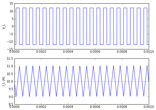
Hey, that's pretty good. From a 24V DC link with 10kHz center-aligned PWM at D = 0.5 and a 150μH inductor, we expected 1.0A peak inductor ripple on top of 10A DC, and we got it right on the nose with our simulation. Now let's see what happens as we increase the DC component of inductor current.
fig = figure(figsize=(8,6),dpi=80)
showIfromV(fig,t2,L1inv,V,psi0list=L1(np.array([12.5,15,17])))
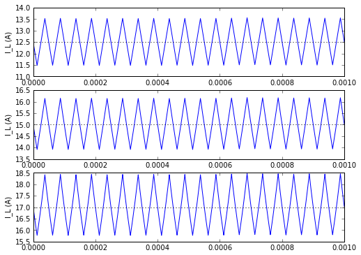
Huh, look at that. The peak-to-peak ripple increases a bit as we go up in DC current. That's about what we'd expect: the inductance drops as we increase DC current, and peak-to-peak ripple is larger with a smaller inductance.
fig = figure(figsize=(8,6),dpi=80)
showIfromV(fig,t2,L1inv,V,psi0list=L1(np.array([18.5,20,21.5])))

You'll note that as the DC current gets larger and larger, the ripple waveform is asymmetric: the positive peak ripple above the DC value is larger than the negative peak ripple, and as we go a bit further, we start to get spiky waveforms. We've gone grossly nonlinear. These last two graphs are driving the inductor very far into saturation.
If you ever see this kind of current waveform on an oscilloscope in a power supply circuit, stop immediately and turn the power supply off. You have exceeded the safe level of current for that inductor. In addition to the inductance dropping and causing larger I2R losses, other nonlinear losses in the magnetic material like hysteresis and eddy currents will increase, and the core material will heat up. I can't find a reference that talks about the temperature coefficient of magnetic saturation flux, but I know that for at least some materials it is negative, which means that as the core heats up, the saturation threshold drops and the ripple effect increases... and you can get thermal runaway. I've had this happen to me once, for a ferrite bobbin core inductor about 2cm in diameter and 2cm in length, and by the time I realized what was going on, the inductor started to smoke and was damaged. It occurred over a timespan of about 10 seconds. I've been told by an experienced power engineer I know that it's slower for larger inductors, but can still occur.
Increases in peak current ripple are also detrimental to overcurrent sensing. It is usually a good idea to have some kind of comparator circuit that prevents the peak current from exceeding an unsafe level. If the amplitude of current ripple is small, then the comparator circuit is directly limiting the low-frequency inductor current. As current ripple gets larger, we have to give up some engineering margin to keep the peak current level below a safe threshold.
Let's look back at that earlier example:
showripple(t,I_Ldc,1.0,T=100e-6)
RMS I_Ldc = 10.019, peak I_Ldc = 14.000
RMS I_L   = 10.035, peak I_L   = 14.997

We had to limit our inductor current so the worst-case peak current is below 15A, for inductor saturation. We based this on a desired sine wave current with 4.5A amplitude on top of 9.5A DC, with worst-case ripple at a duty cycle of 0.5. Remember, peak ripple current amplitude is \( \frac{1}{4}I_R = \frac{1}{4}|D|(1-|D|)I_{R0} \), and for this 150 μH inductor running from a 24V DC link with 10kHz switching, \( I_{R0} = \) 16A, giving us a peak ripple current of 1.0A.
Now let's see what happens if we end up with a different load that doesn't need as much voltage, so we reduce D to 0.2; in this case the peak ripple current decreases to 0.64A, and our peak current is 14.64A. That's good, right? We've got 0.32A of engineering margin left over.
showripple(t,I_Ldc,0.64,T=100e-6)
RMS I_Ldc = 10.019, peak I_Ldc = 14.000
RMS I_L   = 10.025, peak I_L   = 14.637
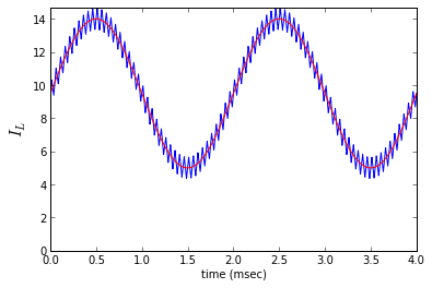
But let's look at our power system from a different angle. We might be controlling this current from an embedded system which gets its current feedback from a current sense circuit. This circuit is based on components which have manufacturing tolerance. Suppose the gain tolerance is ± 2%, so we think we're controlling a low-frequency current \( I_{Ldc} \) which tops out at 14.0A. but could be as high as 14 * 1.02 = 14.28A. What does that look like?
showripple(t,I_Ldc*1.02,0.64,T=100e-6)
RMS I_Ldc = 10.219, peak I_Ldc = 14.280
RMS I_L   = 10.226, peak I_L   = 14.916
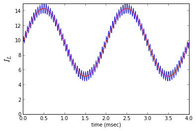
Hmm. It's below the 15A overcurrent threshold, so the peak current is OK, but the RMS current is 10.226A, and that's above the safe limit of 10.1A RMS that we got from our Magnetics Guy. The overcurrent threshold has to be lower if we want to use it to keep RMS current at a safe level.
Here's the lesson: variability in current ripple eats into our design margin. We have to design our magnetics to support peak current at maximum amplitude ripple, but we have to design our overcurrent limits at minimum amplitude ripple if we are trying to use that overcurrent threshold to limit the low-frequency components of current or to limit its RMS value.
Harmonics
Harmonics of ripple current affect radiated and conducted emissions. After all, magnetic components have current-carrying coils that create magnetic fields, and even though most of the fields stay within ferromagnetic material, some of the electromagnetic field "leaks out" into regions outside the magnetic component. If you have a bobbin inductor or air-core inductor, this leakage effect is significant. Most high-power magnetics use a closed magnetic circuit where any magnetic gaps are in the interior of the component, and this minimizes interaction of the magnetic fields with other components. In any case, the lower the ripple, the lower the leakage fields. If you've got a system which has low enough ripple for the magnetic component itself to stay within safe peak and RMS current limits, but it fails EMI testing at harmonics of the switching frequency, you may need to reduce ripple current further.
Ripple current in the DC link capacitors
The important effects of ripple current in the DC link capacitors are a little different:
- The extra RMS current uses up design margin for thermal rise in the capacitor.
- Ripple current in the DC link capacitors causes ripple voltage on the DC link.
RMS current
The RMS current in the capacitor is what causes heating in it. Good capacitors have this RMS current rating listed in their data sheet, and if you're using a serious DC link capacitor for power electronics, you shouldn't use one that doesn't have it shown in the datasheet.
Again, let's go back to the same case as before; our low-frequency load current is 9.5A DC combined with a 4.5A sine wave at 500Hz. The RMS value of the low-frequency current is 10.019A. The RMS load current ripple at the switching frequency varies with duty cycle and is equal to \( I_{Lrms} = \frac{1}{4\sqrt{3}}|D|(1-|D|)I_{R0} \) where \( I_{R0} = \) 16A.
The RMS ripple current in the capacitor, as we figured out in Part II, was \( I_{CDC,rms} = \sqrt{|D|}\sqrt{{I_{Lrms}}^2 + (1-|D|)I_{Ldc}^2} \).
Here's what that RMS capacitor ripple current looks like as a function of duty cycle. We'll just show for positive D; when the load voltage is applied across the load in the other direction for negative D, the results are the same.
def show_rmscap_ripple(I_R0, I_Ldcrms):
  D = np.linspace(0,1,200)
  # RMS of pulse current:
  I_CDCrms_lf = np.sqrt(D*(1-D))*I_Ldcrms
  # RMS of ramp current:
  I_CDCrms_hf = np.sqrt(D)*D*(1-D)*I_R0/4/np.sqrt(3)
  I_CDCrms_total = np.sqrt(I_CDCrms_lf**2 + I_CDCrms_hf**2)
  plt.plot(D,I_CDCrms_lf,D,I_CDCrms_hf,D,I_CDCrms_total)
  plt.xlabel('D')
  plt.ylabel('$RMS(I_{CDC})$',fontsize=15)
  plt.legend(('pulse','ramp','total'))

I_Ldcrms = np.sqrt(9.5**2 + 4.5**2/2)
show_rmscap_ripple(I_R0=16, I_Ldcrms=I_Ldcrms)
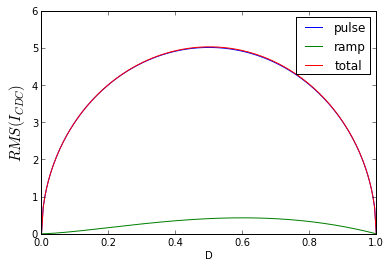
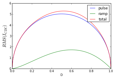
Is that a circle? Yes! The equation for RMS pulse current into the capacitor is \( I_{CDC,RMS} = \sqrt{D(1-D)}I_{Ldcrms} = \sqrt{\frac{1}{2}^2 - (D-\frac{1}{2})^2}I_{Ldcrms} \). Also, the RMS ramp current is small, and has negligible effect on the total RMS capacitor current. Even if we made the RMS ramp current four times larger (4A peak load current ripple), it barely has an effect on the total RMS current:
show_rmscap_ripple(I_R0=64, I_Ldcrms=I_Ldcrms)
Lessons learned:
- Like the RMS load current, the RMS value of DC-link capacitor current ripple is barely affected by load ripple current, unless the ripple current is very large. In most cases, RMS ramp current can be neglected.
- Worst-case RMS pulse current is half of the low-frequency RMS load current, at \( D = \pm\frac{1}{2}. \) In our example, the low-frequency load current is 10.019A; the RMS pulse current in the capacitor is 5.009A.
DC link ripple voltage
We're going to take a look at the ripple voltage on the DC link. The usual assumption about the DC link is that it is, in fact, a DC voltage that is constant, or at most is slowly changing.
The DC link ripple voltage has two sources. One is IR drops from the capacitor's small but nonzero ESR. The other is ΔV from charge transferring in and out of the capacitor.
Let's look at a sample capacitor, the Panasonic TSUP series ECO-S1VP183EA. It's a moderately large electrolytic capacitor: 18000μF ± 20% rated for 35V max, 5.68Arms max at 120Hz, 6.53Arms max @ 10kHz, 30mΩ max at 120Hz, 23mΩ max at 20kHz. It's 35mm in diameter and 35mm in height, about the size of a large marshmallow.
This is just large enough to handle the RMS current in our application. Let's do some analysis to see how large the ripple voltage is. The IR drop from the ESR is easy. Remember those numbers I wanted you to keep handy? Well, it's time to use them. Our peak load current is just about 15A. The peak-to-peak current in the DC link capacitor (remember, it's being chopped at twice the switching frequency with center-aligned PWM) is also this same value, so 15A × 23mΩ = 345mV.
The harder thing to calculate is the ΔV due to the capacitor being charged and discharged. Here we'll turn to Python again.
import matplotlib.pyplot as plt
import numpy as np
import scipy.integrate

def ramp(t): return t % 1
def sawtooth(t): return 1-abs(2*(t % 1) - 1)

def pwm(t,D,centeralign = False):
  '''generate PWM signals with duty cycle D'''
  return ((sawtooth(t) if centeralign else ramp(t)) <= D) * 1.0

def rms(t,y):
    return np.sqrt(np.trapz(y*y,t)/(np.amax(t)-np.amin(t)))

def extendrange(ra,rb):
  '''return a tuple (x1,x2) representing the interval from x1 to x2,
given two input ranges of the same form, or None (representing no input).'''
  if ra is None:
    return rb
  elif rb is None:
    return ra
  else:
    return (min(ra[0],rb[0]),max(ra[1],rb[1]))

def createLimits(margin, *args):
    '''add proportional margin to an interval:
createLimits(0.1, (1,3),(2,4),(0,2)) calculates the maximum extent
of the ranges provided, in this case (0,4), and adds another 0.1 (10%)
to the extent symmetrically, thus returning (-0.2, 4.2).'''
    r = None
    for x in args:
        r = extendrange(r, (np.min(x),np.max(x)))
    rmargin = (r[1]-r[0])*margin/2.0
    return (r[0]-rmargin,r[1]+rmargin)

def calcripple(t,y):
    ''' calculate ripple current by integrating the input,
then adjusting it by a linear function to put both endpoints
at the same value. The slope of the linear function is the
mean value of the input; the offset is chosen to make the mean value
of the output ripple current = 0.'''
    T = t[-1]-t[0]
    yint0 = np.append([0],scipy.integrate.cumtrapz(y,t))
    # cumtrapz produces a vector of length N-1
    # so we need to add one element back in at the beginning
    meanval0 = yint0[-1]/T
    yint1 = yint0 - (t-t[0])*meanval0
    meanval1 = scipy.integrate.trapz(yint1,t)/T
    return yint1 - meanval1

def calc_capacitor_ripple(pwmA,pwmB,I_L,I_S):
    return (pwmA-pwmB)*I_L - I_S

def annotate_level(ax,t,yline,ytext,text,style='k:'):
    tlim = [min(t),max(t)]
    tannot0 = tlim[0] + (tlim[1]-tlim[0])*0.5
    tannot1 = tlim[0] + (tlim[1]-tlim[0])*0.6
    ax.plot(tlim,[yline]*2,style)
    # see:
    # http://matplotlib.org/api/axes_api.html#matplotlib.axes.Axes.annotate
    ax.annotate(text, xy=(tannot0,yline), xytext=(tannot1,ytext),
        bbox=dict(boxstyle="round", fc="0.9"),
        arrowprops=dict(arrowstyle="->",
          connectionstyle="arc,angleA=0,armA=20,angleB=%d,armB=15,rad=7"
             % (-90 if ytext < yline else 90)))

def annotate_ripple(ax,t,Iab,I_Ldc):
    # annotate with peak values
    for y in [min(Iab),max(Iab)]:
      yofs = y-I_Ldc
      annotate_level(ax,t,y,yofs*0.3 + I_Ldc, '$I_{Ldc} %+.5f$' % yofs)

def split_Icdc_2(fig, t, Da, Db, I_Ldc, centeralign=True):
    axlist = []
    pwmA = pwm(t,Da,centeralign)
    pwmB = pwm(t,Db,centeralign)
    I_S = (Da-Db)*I_Ldc
    s = np.sign(Da-Db)
    Iabripple = calcripple(t,pwmA-pwmB)
    Iab = Iabripple + I_Ldc
    Icdc_ramp = calc_capacitor_ripple(pwmA,pwmB,Iabripple,I_S=0)
    Icdc_pulse = I_Ldc*(pwmA-pwmB) - I_S
    Icdc = Icdc_ramp + Icdc_pulse
    Icdc_mean = np.mean(Icdc)

    ax=fig.add_subplot(3,1,1)
    ax.plot(t,Icdc_ramp,t,Iabripple*np.sign(Da-Db),'--r')
    ax.set_ylabel('$I_{CDC\_ramp}$', fontsize=18)
    axlist.append(ax)

    ax=fig.add_subplot(3,1,2)
    ax.plot(t,Icdc_pulse)
    margin = 0.1
    ylim = createLimits(margin, [-I_S,s*I_Ldc-I_S])
    ax.set_ylim(ylim)
    ax.set_ylabel('$I_{CDC\_pulse}$', fontsize=18)
    annotate_level(ax, t, mean(Icdc_pulse), ylim[0]/3, 'mean = %.3f' % mean(Icdc_pulse))
    axlist.append(ax)
    fig.text(0.1,0.5,'+',fontsize=28)

    ax=fig.add_subplot(3,1,3)
    ax.plot(t,Icdc)
    ax.set_ylabel('$I_{CDC}$', fontsize=15)
    annotate_level(ax, t, Icdc_mean, np.min(Icdc)/3, 'mean = %.3f' % (Icdc_mean))
    axlist.append(ax)
    fig.text(0.1,0.22,'=',fontsize=28)

    fig.subplots_adjust(left=0.25, right=0.95)
    return axlist

def split_Qcdc_2(fig, t, Da, Db, I_Ldc, centeralign=True):
    axlist = []
    pwmA = pwm(t,Da,centeralign)
    pwmB = pwm(t,Db,centeralign)
    I_S = (Da-Db)*I_Ldc
    s = np.sign(Da-Db)
    Iabripple = calcripple(t,pwmA-pwmB)
    Iab = Iabripple + I_Ldc
    Icdc_ramp = calc_capacitor_ripple(pwmA,pwmB,Iabripple,I_S=0)
    Icdc_pulse = I_Ldc*(pwmA-pwmB) - I_S
    Icdc = Icdc_ramp + Icdc_pulse
    Icdc_mean = np.mean(Icdc)

    Qcdc_ramp = scipy.integrate.cumtrapz(Icdc_ramp, t, initial=0)
    Qcdc_ramp -= np.mean(Qcdc_ramp)
    Qcdc_pulse = scipy.integrate.cumtrapz(Icdc_pulse, t, initial=0)
    Qcdc = scipy.integrate.cumtrapz(Icdc, t, initial=0)

    ax=fig.add_subplot(3,1,1)
    ax.plot(t,Qcdc_ramp)
    ax.set_ylabel('$Q_{CDC\_ramp}$', fontsize=18)
    axlist.append(ax)

    ax=fig.add_subplot(3,1,2)
    ax.plot(t,Qcdc_pulse)
    margin = 0.1
    ax.set_ylabel('$Q_{CDC\_pulse}$', fontsize=18)
    axlist.append(ax)
    fig.text(0.1,0.5,'+',fontsize=28)

    ax=fig.add_subplot(3,1,3)
    ax.plot(t,Qcdc)
    ax.set_ylabel('$Q_{CDC}$', fontsize=15)
    axlist.append(ax)
    fig.text(0.1,0.22,'=',fontsize=28)

    fig.subplots_adjust(left=0.25, right=0.95)
    return axlist

t = np.arange(0,4,0.0001)
fig = plt.figure(figsize=(8, 6), dpi=80)
ha = split_Icdc_2(fig, t, 0.7, 0.1, I_Ldc=1.0, centeralign=True)
ha[0].set_title('$I_{CDC}/I_{R0}$ for $D_a=0.7, D_b=0.1, I_{Ldc}=I_{R0}$',fontsize=16)
fig2 = plt.figure(figsize=(8, 6), dpi=80)
ha=split_Qcdc_2(fig2, t, 0.7, 0.1, I_Ldc=1.0, centeralign=True)
ha[0].set_title('$Q_{CDC}/I_{R0}T$ for $D_a=0.7, D_b=0.1, I_{Ldc}=I_{R0}$',fontsize=16)
fig3 = plt.figure(figsize=(8, 6), dpi=80)
ha=split_Icdc_2(fig3, t, 0.75, 0.25, I_Ldc=0.875, centeralign=True)
ha[0].set_title('$I_{CDC}/I_{R0}$ for $D_a=0.75, D_b=0.25, I_{Ldc}=0.875I_{R0}$',fontsize=16)
fig4 = plt.figure(figsize=(8, 6), dpi=80)
ha=split_Qcdc_2(fig4, t, 0.75, 0.25, I_Ldc=0.875, centeralign=True)
ha[0].set_title('$Q_{CDC}/I_{R0}T$ for $D_a=0.75, D_b=0.25, I_{Ldc}=0.875I_{R0}$',fontsize=16)
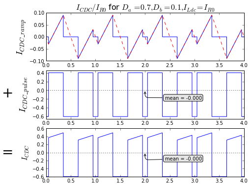
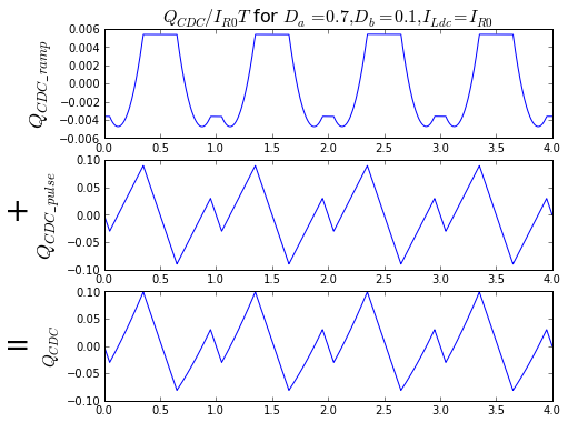
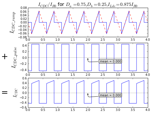
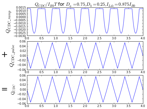
Ignore the numbers here and just pay attention to the wave shapes. The ramp portion of capacitor ripple current affects the capacitor charge ripple very little; for the most part the pulse portion of capacitor ripple current dominates.
To actually analyze this as a general function of duty cycles is a little bit tricky. But the good news is that to figure out peak-to-peak charge variation, we can just look at the longer time interval where the load is short-circuited: the ramp current is zero, and the pulse current is \( -DI _ {Ldc} \) for time period \( \Delta T \), where (and I'm going to skip a few steps here, just trust my algebra)
$$\begin{eqnarray} \Delta T &=& \max(\min(D _ a,1-D _ a),\min(D _ b,1-D _ b))T \cr &=& \frac{1-|D|+|2D _ 0 - 1|}{2}T \end{eqnarray}$$
So we can write $$\begin{eqnarray} \Delta V _ {DC} &=& \frac{\Delta Q _ {DC}}{C _ {DC}} \cr &=& \frac{DI _ {Ldc}T}{2C _ {DC}}(1-|D| + |2D_0 - 1|) \end{eqnarray}$$
For our Panasonic ECO-S1VP183EA 18000μF +/- 20% capacitor under our example scenario, if we plug in the numbers, \( 2D_0-1 = 0 \) (the best case for minimizing current ripple in an H-bridge), and this simplifies to \( \Delta V = \frac{D (1-|D|) I _ {Ldc}}{2C _ {DC}} = 1/8 \times 14A \times 100\mu s / (18000 * 0.8) = 12.2mV \). Compare that to the 345mV due to ESR.
There are some lessons here:
-
Typical DC link voltage ripple in switching converters, in the kilohertz switching frequency and above, is generally dominated by the ESR of the capacitor and not the capacitance itself.
-
You can calculate the DC voltage ripple! It's not hard if you have these equations, and if we look at the numbers, 12mV + 345mV = 357mV is not much ripple on a 24V link. The assumption that the DC link voltage is reasonably constant, at least in this case, is a good assumption.
Summary
Yay! It's that time again! What have we learned today?
-
Make sure your H-bridge's load can handle the RMS current and the peak current.
-
For peak current, don't forget to include the ripple current caused by PWM switching.
-
RMS current due to PWM switching ripple is rarely a problem; it's a very small contribution (usually under 1%) unless the switching ripple is huge.
-
Peak current is important to keep the load inductance out of saturation.
-
Limiting RMS current in the DC link capacitor is important to keep the capacitor cool.
-
As long as switching ripple is not large, RMS current in the DC link capacitor is at most half of the RMS load current.
-
Peak DC link voltage ripple has two parts:
- IR drop due to DC link capacitor ESR is equal to ESR × maximum load current (including switching ripple)
-
ΔV due to capacitor charging/discharging is dominated by the pulse portion of capacitor current (effects from switching ripple can usually be neglected) and can be calculated from the operating point values.
-
ESR is usually the main contributor to the DC link voltage ripple, with the ΔV term often much smaller.
-
You can calculate all these values yourself!
OK, that's all for now. Our last part of this series will talk a little bit about DC link capacitors, layout, parts placement, and why electrolytic capacitors are usually Not Enough.
Happy switching!
© 2013 Jason M. Sachs, all rights reserved.
Stay tuned for a link to this code in an IPython Notebook. I'll put it up on the web, and I do plan to release this in an open-source license, I just have to do a little more homework before I pick the right one.
- Comments
- Write a Comment Select to add a comment
Have you published the last part in the H-Bridge series?
Thanks,
Steve


Lots of effort , nice work,
Thanks
To post reply to a comment, click on the 'reply' button attached to each comment. To post a new comment (not a reply to a comment) check out the 'Write a Comment' tab at the top of the comments.
Please login (on the right) if you already have an account on this platform.
Otherwise, please use this form to register (free) an join one of the largest online community for Electrical/Embedded/DSP/FPGA/ML engineers:


