

On 7/27/2014 11:48 PM, John Larkin wrote:> On Sun, 27 Jul 2014 19:26:57 -0700, RobertMacy <robert.a.macy@gmail.com> wrote: > >> here is the LTspice schematic showing the diffiuclty at 'calibrating' your >> noise source. >> >> Version 4 >> SHEET 1 27404 860 >> WIRE 1984 -336 1808 -336 >> WIRE 2096 -336 1984 -336 >> WIRE 2128 -336 2096 -336 >> WIRE 1808 -304 1808 -336 >> WIRE 1984 -304 1984 -336 >> WIRE 1808 -192 1808 -224 >> WIRE 1984 -192 1984 -224 >> FLAG 1984 -192 0 >> FLAG 1808 -192 0 >> FLAG 2096 -336 noise >> SYMBOL res 1968 -320 R0 >> SYMATTR InstName R1 >> SYMATTR Value 1 >> SYMBOL bv 1808 -320 R0 >> WINDOW 0 -67 10 Left 2 >> WINDOW 3 -414 168 Left 2 >> SYMATTR InstName B1 >> SYMATTR Value V=(random(100*time)-0.5)/0.20353/1.134/0.98523 >> TEXT 1448 -272 Left 2 !.tran 5 >> TEXT 1448 -336 Left 2 !.options plotwinsize=0;\n.param fmax=50 >> TEXT 2256 -312 Left 2 ;Why does it take three attempts to find the >> constant to make this 1Vrms?\nV=random(100*time)-0.5 produces >> 203.53mVrms\nV=(random(100*time)-0.5)/0.20353 produces >> 1.134Vrms\nV=(random(100*time)-0.5)/0.20353/1.134 produces >> 985.23mVrms\nV=(random(100*time)-0.5)/0.20353/1.134/0.98523 produces >> 1.0005Vrms\nnote: k=4.3977, not the expected sqrt(12)=3.4641, odd. >> TEXT 1704 -408 Left 3 ;Uncontrollable Aspects of Using Random Function as >> a Noise Source >> >> >> >> oops, guess it wasn't that long! > > > The problem here is that, with only one simple function on the screen, LT Spice > uses huge time steps and gets the RMS value wrong. LT Spice is quirky that way. > I wish it allowed me to specify the exact, invariant time step; that would help > with a number of issues. > > Try setting the max time step to 10u or 100u. Then things scale sensibly. The > correct RMS value of 'noise', unscaled, seems to be 251.1 mV. > >You can also use a Box-Mueller transform to get independent Gaussian noise sources (see below). There are some odd FFT effects. If you run it for 8 seconds with .options plotwinsize=0, the vanilla trapezoid method, the default time stepping behaviour, and the longest available FFT, you get right around -40 dBV out to about 1 kHz, at which point it drops to about -48 dBV. If you run it for a bit over two seconds with all compression turned off, the FFT starts out at about -24 dBV and drops to about -45 dBV between 300 Hz and 3 kHz. Finer details are hard to recognize, because in an FFT of noise, the variance equals the mean unless you average scans or do frequency binning. Some extra work will be required to get this method to be a reliable noise source for transient analysis. Of course a variable-stepsize simulation will require that the data be resampled before it can do an FFT, so it's unclear whether the artifacts are coming from the transient simulation or the transform calculation. I also still doubt very much whether op amp macromodels are going to do the right thing when they go nonlinear. Cheers Phil Hobbs Version 4 SHEET 1 1656 900 WIRE -224 192 -256 192 WIRE -224 208 -224 192 WIRE 144 304 128 304 WIRE 384 304 368 304 WIRE -224 320 -224 288 WIRE 128 352 128 304 WIRE 368 352 368 304 WIRE -240 400 -256 400 WIRE -240 416 -240 400 WIRE 128 464 128 432 WIRE 368 464 368 432 WIRE -240 512 -240 496 FLAG 128 464 0 FLAG 144 304 n1 FLAG 368 464 0 FLAG 384 304 n2 FLAG -240 512 0 FLAG -224 320 0 FLAG -256 400 gn1 FLAG -256 192 gn2 SYMBOL bv 128 336 R0 SYMATTR InstName B2 SYMATTR Value V=rand(50000*time) SYMBOL bv 368 336 R0 SYMATTR InstName B1 SYMATTR Value V=rand(50000*time-20000) SYMBOL bv -240 400 R0 SYMATTR InstName B3 SYMATTR Value V=sqrt(-2*ln(v(n2)))*cos(2*pi*v(n1)) SYMBOL bv -224 192 R0 WINDOW 3 60 49 Left 2 SYMATTR InstName B4 SYMATTR Value V=sqrt(-2*ln(v(n2)))*sin(2*pi*v(n1)) TEXT 208 368 Left 2 !.tran 8m -- Dr Philip C D Hobbs Principal Consultant ElectroOptical Innovations LLC Optics, Electro-optics, Photonics, Analog Electronics 160 North State Road #203 Briarcliff Manor NY 10510 hobbs at electrooptical dot net http://electrooptical.net
Learning about oscillators in LTSpice
Started by ●October 21, 2010
Reply by ●July 28, 20142014-07-28
Reply by ●July 28, 20142014-07-28
On Mon, 28 Jul 2014 07:58:07 -0700, Phil Hobbs <hobbs@electrooptical.net> wrote:>> ...snip... > I also still doubt very much whether op amp macromodels are going to do > the right thing when they go nonlinear. > > Cheers > > Phil Hobbs > ...snip....Thanks for jumping in, Phil. That is ABSOLUTELY true!!! Using simple minded pair of input current noise sources and a single input voltage noise source only work within approximately 1/2 the CLOSED loop bandwidth for obvious reasons. AND, they don't work if the OpAmp pops out of linear behaviour, again for obvious reasons. However still interesting if you're designing a receiver, or pre-amp. Jim Thompson's OpAmp model with resistor and transistor noise sources stuck in into a few judicious places does seem to get much closer to simulating over much wider conditions, like out of bandwidth and into slew rate limit. So as usual, complexity versus accuracy is the trade off.
Reply by ●July 28, 20142014-07-28
On 7/28/2014 11:17 AM, RobertMacy wrote:> On Mon, 28 Jul 2014 07:58:07 -0700, Phil Hobbs > <hobbs@electrooptical.net> wrote: > >>> ...snip... >> I also still doubt very much whether op amp macromodels are going to >> do the right thing when they go nonlinear. >> >> Cheers >> >> Phil Hobbs >> ...snip.... > > Thanks for jumping in, Phil. > > That is ABSOLUTELY true!!! > > Using simple minded pair of input current noise sources and a single > input voltage noise source only work within approximately 1/2 the CLOSED > loop bandwidth for obvious reasons. AND, they don't work if the OpAmp > pops out of linear behaviour, again for obvious reasons. However still > interesting if you're designing a receiver, or pre-amp. > > Jim Thompson's OpAmp model with resistor and transistor noise sources > stuck in into a few judicious places does seem to get much closer to > simulating over much wider conditions, like out of bandwidth and into > slew rate limit. So as usual, complexity versus accuracy is the trade off.It turns out that the default behaviour is pretty sensible if you pick the right parameters. Using the vanilla trapezoid with maxstep = 1u and all compression turned off, a transient of 2.097152 s (2**22 data points at maximum time resolution) comes out with a pretty flat spectrum that looks pretty much exactly as you'd expect. 1 VRMS with a 50 kHz bandwidth is -47 dBV/Hz, which (by eyeball accuracy) is what you actually get. The random staircase function shows the expected sinc function rolloff with a first null at 50 kHz. So it looks like there is no major impediment to using this method, as long as you keep Mike from getting too clever on you. ;) Cheers Phil Hobbs -- Dr Philip C D Hobbs Principal Consultant ElectroOptical Innovations LLC Optics, Electro-optics, Photonics, Analog Electronics 160 North State Road #203 Briarcliff Manor NY 10510 hobbs at electrooptical dot net http://electrooptical.net
Reply by ●July 28, 20142014-07-28
On Mon, 28 Jul 2014 10:58:07 -0400, Phil Hobbs <hobbs@electrooptical.net> wrote:>On 7/27/2014 11:48 PM, John Larkin wrote: >> On Sun, 27 Jul 2014 19:26:57 -0700, RobertMacy <robert.a.macy@gmail.com> wrote: >> >>> here is the LTspice schematic showing the diffiuclty at 'calibrating' your >>> noise source. >>> >>> Version 4 >>> SHEET 1 27404 860 >>> WIRE 1984 -336 1808 -336 >>> WIRE 2096 -336 1984 -336 >>> WIRE 2128 -336 2096 -336 >>> WIRE 1808 -304 1808 -336 >>> WIRE 1984 -304 1984 -336 >>> WIRE 1808 -192 1808 -224 >>> WIRE 1984 -192 1984 -224 >>> FLAG 1984 -192 0 >>> FLAG 1808 -192 0 >>> FLAG 2096 -336 noise >>> SYMBOL res 1968 -320 R0 >>> SYMATTR InstName R1 >>> SYMATTR Value 1 >>> SYMBOL bv 1808 -320 R0 >>> WINDOW 0 -67 10 Left 2 >>> WINDOW 3 -414 168 Left 2 >>> SYMATTR InstName B1 >>> SYMATTR Value V=(random(100*time)-0.5)/0.20353/1.134/0.98523 >>> TEXT 1448 -272 Left 2 !.tran 5 >>> TEXT 1448 -336 Left 2 !.options plotwinsize=0;\n.param fmax=50 >>> TEXT 2256 -312 Left 2 ;Why does it take three attempts to find the >>> constant to make this 1Vrms?\nV=random(100*time)-0.5 produces >>> 203.53mVrms\nV=(random(100*time)-0.5)/0.20353 produces >>> 1.134Vrms\nV=(random(100*time)-0.5)/0.20353/1.134 produces >>> 985.23mVrms\nV=(random(100*time)-0.5)/0.20353/1.134/0.98523 produces >>> 1.0005Vrms\nnote: k=4.3977, not the expected sqrt(12)=3.4641, odd. >>> TEXT 1704 -408 Left 3 ;Uncontrollable Aspects of Using Random Function as >>> a Noise Source >>> >>> >>> >>> oops, guess it wasn't that long! >> >> >> The problem here is that, with only one simple function on the screen, LT Spice >> uses huge time steps and gets the RMS value wrong. LT Spice is quirky that way. >> I wish it allowed me to specify the exact, invariant time step; that would help >> with a number of issues. >> >> Try setting the max time step to 10u or 100u. Then things scale sensibly. The >> correct RMS value of 'noise', unscaled, seems to be 251.1 mV. >> >> > >You can also use a Box-Mueller transform to get independent Gaussian >noise sources (see below). > > >There are some odd FFT effects. If you run it for 8 seconds with >.options plotwinsize=0, the vanilla trapezoid method, the default time >stepping behaviour, and the longest available FFT, you get right around >-40 dBV out to about 1 kHz, at which point it drops to about -48 dBV. >If you run it for a bit over two seconds with all compression turned >off, the FFT starts out at about -24 dBV and drops to about -45 dBV >between 300 Hz and 3 kHz. > >Finer details are hard to recognize, because in an FFT of noise, the >variance equals the mean unless you average scans or do frequency binning. > >Some extra work will be required to get this method to be a reliable >noise source for transient analysis. Of course a variable-stepsize >simulation will require that the data be resampled before it can do an >FFT, so it's unclear whether the artifacts are coming from the transient >simulation or the transform calculation. > >I also still doubt very much whether op amp macromodels are going to do >the right thing when they go nonlinear. > >Cheers > >Phil Hobbs > >Version 4 >SHEET 1 1656 900 >WIRE -224 192 -256 192 >WIRE -224 208 -224 192 >WIRE 144 304 128 304 >WIRE 384 304 368 304 >WIRE -224 320 -224 288 >WIRE 128 352 128 304 >WIRE 368 352 368 304 >WIRE -240 400 -256 400 >WIRE -240 416 -240 400 >WIRE 128 464 128 432 >WIRE 368 464 368 432 >WIRE -240 512 -240 496 >FLAG 128 464 0 >FLAG 144 304 n1 >FLAG 368 464 0 >FLAG 384 304 n2 >FLAG -240 512 0 >FLAG -224 320 0 >FLAG -256 400 gn1 >FLAG -256 192 gn2 >SYMBOL bv 128 336 R0 >SYMATTR InstName B2 >SYMATTR Value V=rand(50000*time) >SYMBOL bv 368 336 R0 >SYMATTR InstName B1 >SYMATTR Value V=rand(50000*time-20000) >SYMBOL bv -240 400 R0 >SYMATTR InstName B3 >SYMATTR Value V=sqrt(-2*ln(v(n2)))*cos(2*pi*v(n1)) >SYMBOL bv -224 192 R0 >WINDOW 3 60 49 Left 2 >SYMATTR InstName B4 >SYMATTR Value V=sqrt(-2*ln(v(n2)))*sin(2*pi*v(n1)) >TEXT 208 368 Left 2 !.tran 8mrand(time) and random(time) do make different spectra (expected) and different RMS values (unexpected?) because of the soft transitions of 'random.' I can't imagine what might be the algorithm for those transitions. -- John Larkin Highland Technology Inc www.highlandtechnology.com jlarkin at highlandtechnology dot com Precision electronic instrumentation
Reply by ●July 28, 20142014-07-28
On 7/28/2014 12:01 PM, John Larkin wrote:> On Mon, 28 Jul 2014 10:58:07 -0400, Phil Hobbs <hobbs@electrooptical.net> wrote: > >> On 7/27/2014 11:48 PM, John Larkin wrote: >>> On Sun, 27 Jul 2014 19:26:57 -0700, RobertMacy <robert.a.macy@gmail.com> wrote: >>> >>>> here is the LTspice schematic showing the diffiuclty at 'calibrating' your >>>> noise source. >>>> >>>> Version 4 >>>> SHEET 1 27404 860 >>>> WIRE 1984 -336 1808 -336 >>>> WIRE 2096 -336 1984 -336 >>>> WIRE 2128 -336 2096 -336 >>>> WIRE 1808 -304 1808 -336 >>>> WIRE 1984 -304 1984 -336 >>>> WIRE 1808 -192 1808 -224 >>>> WIRE 1984 -192 1984 -224 >>>> FLAG 1984 -192 0 >>>> FLAG 1808 -192 0 >>>> FLAG 2096 -336 noise >>>> SYMBOL res 1968 -320 R0 >>>> SYMATTR InstName R1 >>>> SYMATTR Value 1 >>>> SYMBOL bv 1808 -320 R0 >>>> WINDOW 0 -67 10 Left 2 >>>> WINDOW 3 -414 168 Left 2 >>>> SYMATTR InstName B1 >>>> SYMATTR Value V=(random(100*time)-0.5)/0.20353/1.134/0.98523 >>>> TEXT 1448 -272 Left 2 !.tran 5 >>>> TEXT 1448 -336 Left 2 !.options plotwinsize=0;\n.param fmax=50 >>>> TEXT 2256 -312 Left 2 ;Why does it take three attempts to find the >>>> constant to make this 1Vrms?\nV=random(100*time)-0.5 produces >>>> 203.53mVrms\nV=(random(100*time)-0.5)/0.20353 produces >>>> 1.134Vrms\nV=(random(100*time)-0.5)/0.20353/1.134 produces >>>> 985.23mVrms\nV=(random(100*time)-0.5)/0.20353/1.134/0.98523 produces >>>> 1.0005Vrms\nnote: k=4.3977, not the expected sqrt(12)=3.4641, odd. >>>> TEXT 1704 -408 Left 3 ;Uncontrollable Aspects of Using Random Function as >>>> a Noise Source >>>> >>>> >>>> >>>> oops, guess it wasn't that long! >>> >>> >>> The problem here is that, with only one simple function on the screen, LT Spice >>> uses huge time steps and gets the RMS value wrong. LT Spice is quirky that way. >>> I wish it allowed me to specify the exact, invariant time step; that would help >>> with a number of issues. >>> >>> Try setting the max time step to 10u or 100u. Then things scale sensibly. The >>> correct RMS value of 'noise', unscaled, seems to be 251.1 mV. >>> >>> >> >> You can also use a Box-Mueller transform to get independent Gaussian >> noise sources (see below). >> >> >> There are some odd FFT effects. If you run it for 8 seconds with >> .options plotwinsize=0, the vanilla trapezoid method, the default time >> stepping behaviour, and the longest available FFT, you get right around >> -40 dBV out to about 1 kHz, at which point it drops to about -48 dBV. >> If you run it for a bit over two seconds with all compression turned >> off, the FFT starts out at about -24 dBV and drops to about -45 dBV >> between 300 Hz and 3 kHz. >> >> Finer details are hard to recognize, because in an FFT of noise, the >> variance equals the mean unless you average scans or do frequency binning. >> >> Some extra work will be required to get this method to be a reliable >> noise source for transient analysis. Of course a variable-stepsize >> simulation will require that the data be resampled before it can do an >> FFT, so it's unclear whether the artifacts are coming from the transient >> simulation or the transform calculation. >> >> I also still doubt very much whether op amp macromodels are going to do >> the right thing when they go nonlinear. >> >> Cheers >> >> Phil Hobbs >> >> Version 4 >> SHEET 1 1656 900 >> WIRE -224 192 -256 192 >> WIRE -224 208 -224 192 >> WIRE 144 304 128 304 >> WIRE 384 304 368 304 >> WIRE -224 320 -224 288 >> WIRE 128 352 128 304 >> WIRE 368 352 368 304 >> WIRE -240 400 -256 400 >> WIRE -240 416 -240 400 >> WIRE 128 464 128 432 >> WIRE 368 464 368 432 >> WIRE -240 512 -240 496 >> FLAG 128 464 0 >> FLAG 144 304 n1 >> FLAG 368 464 0 >> FLAG 384 304 n2 >> FLAG -240 512 0 >> FLAG -224 320 0 >> FLAG -256 400 gn1 >> FLAG -256 192 gn2 >> SYMBOL bv 128 336 R0 >> SYMATTR InstName B2 >> SYMATTR Value V=rand(50000*time) >> SYMBOL bv 368 336 R0 >> SYMATTR InstName B1 >> SYMATTR Value V=rand(50000*time-20000) >> SYMBOL bv -240 400 R0 >> SYMATTR InstName B3 >> SYMATTR Value V=sqrt(-2*ln(v(n2)))*cos(2*pi*v(n1)) >> SYMBOL bv -224 192 R0 >> WINDOW 3 60 49 Left 2 >> SYMATTR InstName B4 >> SYMATTR Value V=sqrt(-2*ln(v(n2)))*sin(2*pi*v(n1)) >> TEXT 208 368 Left 2 !.tran 8m > > rand(time) and random(time) do make different spectra (expected) and different > RMS values (unexpected?) because of the soft transitions of 'random.' I can't > imagine what might be the algorithm for those transitions. > >Probably tanh() or atan(). Mike uses atan() for his soft switches. Cheers Phil Hobbs -- Dr Philip C D Hobbs Principal Consultant ElectroOptical Innovations LLC Optics, Electro-optics, Photonics, Analog Electronics 160 North State Road #203 Briarcliff Manor NY 10510 hobbs at electrooptical dot net http://electrooptical.net
Reply by ●July 28, 20142014-07-28
"RobertMacy" wrote in message news:op.xjk63sru2cx0wh@ajm...>>> and worst of all!!! put two in your circuit and they both produce the >>> SAME >>> voltage!!! just like white() does. > >> Then change the time scalers. Change the amplitudes. Sum a few to make >> things more Gaussian... there might even be a theorem about that.>Change in some arbitrary manner? No way! Again, what I do is CALIBRATED, >so the results have value. The technique to get .tranoise is TRUE circuit >simulation where in one pass you get BOTH .noise and .tranI would guess that you could also figure out how in just one pass, I get SuperSpice to figure out the values of all the resisters and mosfet sizes to achieve a a specified set of voltages and currents. Standard optimisers iterate out the results. http://www.anasoft.co.uk/devicedesigner.htm Kevin Aylward www.kevinaylward.co.uk www.anasoft.co.uk - SuperSpice
Reply by ●July 28, 20142014-07-28
On Mon, 28 Jul 2014 12:08:49 -0400, Phil Hobbs <hobbs@electrooptical.net> wrote:>On 7/28/2014 12:01 PM, John Larkin wrote: >> On Mon, 28 Jul 2014 10:58:07 -0400, Phil Hobbs <hobbs@electrooptical.net> wrote: >> >>> On 7/27/2014 11:48 PM, John Larkin wrote: >>>> On Sun, 27 Jul 2014 19:26:57 -0700, RobertMacy <robert.a.macy@gmail.com> wrote: >>>> >>>>> here is the LTspice schematic showing the diffiuclty at 'calibrating' your >>>>> noise source. >>>>> >>>>> Version 4 >>>>> SHEET 1 27404 860 >>>>> WIRE 1984 -336 1808 -336 >>>>> WIRE 2096 -336 1984 -336 >>>>> WIRE 2128 -336 2096 -336 >>>>> WIRE 1808 -304 1808 -336 >>>>> WIRE 1984 -304 1984 -336 >>>>> WIRE 1808 -192 1808 -224 >>>>> WIRE 1984 -192 1984 -224 >>>>> FLAG 1984 -192 0 >>>>> FLAG 1808 -192 0 >>>>> FLAG 2096 -336 noise >>>>> SYMBOL res 1968 -320 R0 >>>>> SYMATTR InstName R1 >>>>> SYMATTR Value 1 >>>>> SYMBOL bv 1808 -320 R0 >>>>> WINDOW 0 -67 10 Left 2 >>>>> WINDOW 3 -414 168 Left 2 >>>>> SYMATTR InstName B1 >>>>> SYMATTR Value V=(random(100*time)-0.5)/0.20353/1.134/0.98523 >>>>> TEXT 1448 -272 Left 2 !.tran 5 >>>>> TEXT 1448 -336 Left 2 !.options plotwinsize=0;\n.param fmax=50 >>>>> TEXT 2256 -312 Left 2 ;Why does it take three attempts to find the >>>>> constant to make this 1Vrms?\nV=random(100*time)-0.5 produces >>>>> 203.53mVrms\nV=(random(100*time)-0.5)/0.20353 produces >>>>> 1.134Vrms\nV=(random(100*time)-0.5)/0.20353/1.134 produces >>>>> 985.23mVrms\nV=(random(100*time)-0.5)/0.20353/1.134/0.98523 produces >>>>> 1.0005Vrms\nnote: k=4.3977, not the expected sqrt(12)=3.4641, odd. >>>>> TEXT 1704 -408 Left 3 ;Uncontrollable Aspects of Using Random Function as >>>>> a Noise Source >>>>> >>>>> >>>>> >>>>> oops, guess it wasn't that long! >>>> >>>> >>>> The problem here is that, with only one simple function on the screen, LT Spice >>>> uses huge time steps and gets the RMS value wrong. LT Spice is quirky that way. >>>> I wish it allowed me to specify the exact, invariant time step; that would help >>>> with a number of issues. >>>> >>>> Try setting the max time step to 10u or 100u. Then things scale sensibly. The >>>> correct RMS value of 'noise', unscaled, seems to be 251.1 mV. >>>> >>>> >>> >>> You can also use a Box-Mueller transform to get independent Gaussian >>> noise sources (see below). >>> >>> >>> There are some odd FFT effects. If you run it for 8 seconds with >>> .options plotwinsize=0, the vanilla trapezoid method, the default time >>> stepping behaviour, and the longest available FFT, you get right around >>> -40 dBV out to about 1 kHz, at which point it drops to about -48 dBV. >>> If you run it for a bit over two seconds with all compression turned >>> off, the FFT starts out at about -24 dBV and drops to about -45 dBV >>> between 300 Hz and 3 kHz. >>> >>> Finer details are hard to recognize, because in an FFT of noise, the >>> variance equals the mean unless you average scans or do frequency binning. >>> >>> Some extra work will be required to get this method to be a reliable >>> noise source for transient analysis. Of course a variable-stepsize >>> simulation will require that the data be resampled before it can do an >>> FFT, so it's unclear whether the artifacts are coming from the transient >>> simulation or the transform calculation. >>> >>> I also still doubt very much whether op amp macromodels are going to do >>> the right thing when they go nonlinear. >>> >>> Cheers >>> >>> Phil Hobbs >>> >>> Version 4 >>> SHEET 1 1656 900 >>> WIRE -224 192 -256 192 >>> WIRE -224 208 -224 192 >>> WIRE 144 304 128 304 >>> WIRE 384 304 368 304 >>> WIRE -224 320 -224 288 >>> WIRE 128 352 128 304 >>> WIRE 368 352 368 304 >>> WIRE -240 400 -256 400 >>> WIRE -240 416 -240 400 >>> WIRE 128 464 128 432 >>> WIRE 368 464 368 432 >>> WIRE -240 512 -240 496 >>> FLAG 128 464 0 >>> FLAG 144 304 n1 >>> FLAG 368 464 0 >>> FLAG 384 304 n2 >>> FLAG -240 512 0 >>> FLAG -224 320 0 >>> FLAG -256 400 gn1 >>> FLAG -256 192 gn2 >>> SYMBOL bv 128 336 R0 >>> SYMATTR InstName B2 >>> SYMATTR Value V=rand(50000*time) >>> SYMBOL bv 368 336 R0 >>> SYMATTR InstName B1 >>> SYMATTR Value V=rand(50000*time-20000) >>> SYMBOL bv -240 400 R0 >>> SYMATTR InstName B3 >>> SYMATTR Value V=sqrt(-2*ln(v(n2)))*cos(2*pi*v(n1)) >>> SYMBOL bv -224 192 R0 >>> WINDOW 3 60 49 Left 2 >>> SYMATTR InstName B4 >>> SYMATTR Value V=sqrt(-2*ln(v(n2)))*sin(2*pi*v(n1)) >>> TEXT 208 368 Left 2 !.tran 8m >> >> rand(time) and random(time) do make different spectra (expected) and different >> RMS values (unexpected?) because of the soft transitions of 'random.' I can't >> imagine what might be the algorithm for those transitions. >> >> >Probably tanh() or atan(). Mike uses atan() for his soft switches. > >Cheers > >Phil HobbsIf I do random(time), the transition shape is independent of the sim dt. If I do random(99*time) the shape is scaled in time but looks the same. So random() is aware of the '99'. Somehow. Maybe it remembers the time of the previous invocation. Mike must have all sorts of tricks in there. -- John Larkin Highland Technology Inc www.highlandtechnology.com jlarkin at highlandtechnology dot com Precision electronic instrumentation
Reply by ●July 28, 20142014-07-28
On Mon, 28 Jul 2014 12:08:49 -0400, Phil Hobbs <hobbs@electrooptical.net> wrote: [snip]>> >> rand(time) and random(time) do make different spectra (expected) and different >> RMS values (unexpected?) because of the soft transitions of 'random.' I can't >> imagine what might be the algorithm for those transitions. >> >> >Probably tanh() or atan(). Mike uses atan() for his soft switches. > >Cheers > >Phil HobbsI use TANH for my switches... G-sources, switching from low to high conductance... works quite nicely with no convergence issues. ...Jim Thompson -- | James E.Thompson | mens | | Analog Innovations | et | | Analog/Mixed-Signal ASIC's and Discrete Systems | manus | | San Tan Valley, AZ 85142 Skype: skypeanalog | | | Voice:(480)460-2350 Fax: Available upon request | Brass Rat | | E-mail Icon at http://www.analog-innovations.com | 1962 | I love to cook with wine. Sometimes I even put it in the food.
Reply by ●July 28, 20142014-07-28
On 7/28/2014 12:47 PM, John Larkin wrote:> On Mon, 28 Jul 2014 12:08:49 -0400, Phil Hobbs <hobbs@electrooptical.net> wrote: > >> On 7/28/2014 12:01 PM, John Larkin wrote: >>> On Mon, 28 Jul 2014 10:58:07 -0400, Phil Hobbs <hobbs@electrooptical.net> wrote: >>> >>>> On 7/27/2014 11:48 PM, John Larkin wrote: >>>>> On Sun, 27 Jul 2014 19:26:57 -0700, RobertMacy <robert.a.macy@gmail.com> wrote: >>>>> >>>>>> here is the LTspice schematic showing the diffiuclty at 'calibrating' your >>>>>> noise source. >>>>>> >>>>>> Version 4 >>>>>> SHEET 1 27404 860 >>>>>> WIRE 1984 -336 1808 -336 >>>>>> WIRE 2096 -336 1984 -336 >>>>>> WIRE 2128 -336 2096 -336 >>>>>> WIRE 1808 -304 1808 -336 >>>>>> WIRE 1984 -304 1984 -336 >>>>>> WIRE 1808 -192 1808 -224 >>>>>> WIRE 1984 -192 1984 -224 >>>>>> FLAG 1984 -192 0 >>>>>> FLAG 1808 -192 0 >>>>>> FLAG 2096 -336 noise >>>>>> SYMBOL res 1968 -320 R0 >>>>>> SYMATTR InstName R1 >>>>>> SYMATTR Value 1 >>>>>> SYMBOL bv 1808 -320 R0 >>>>>> WINDOW 0 -67 10 Left 2 >>>>>> WINDOW 3 -414 168 Left 2 >>>>>> SYMATTR InstName B1 >>>>>> SYMATTR Value V=(random(100*time)-0.5)/0.20353/1.134/0.98523 >>>>>> TEXT 1448 -272 Left 2 !.tran 5 >>>>>> TEXT 1448 -336 Left 2 !.options plotwinsize=0;\n.param fmax=50 >>>>>> TEXT 2256 -312 Left 2 ;Why does it take three attempts to find the >>>>>> constant to make this 1Vrms?\nV=random(100*time)-0.5 produces >>>>>> 203.53mVrms\nV=(random(100*time)-0.5)/0.20353 produces >>>>>> 1.134Vrms\nV=(random(100*time)-0.5)/0.20353/1.134 produces >>>>>> 985.23mVrms\nV=(random(100*time)-0.5)/0.20353/1.134/0.98523 produces >>>>>> 1.0005Vrms\nnote: k=4.3977, not the expected sqrt(12)=3.4641, odd. >>>>>> TEXT 1704 -408 Left 3 ;Uncontrollable Aspects of Using Random Function as >>>>>> a Noise Source >>>>>> >>>>>> >>>>>> >>>>>> oops, guess it wasn't that long! >>>>> >>>>> >>>>> The problem here is that, with only one simple function on the screen, LT Spice >>>>> uses huge time steps and gets the RMS value wrong. LT Spice is quirky that way. >>>>> I wish it allowed me to specify the exact, invariant time step; that would help >>>>> with a number of issues. >>>>> >>>>> Try setting the max time step to 10u or 100u. Then things scale sensibly. The >>>>> correct RMS value of 'noise', unscaled, seems to be 251.1 mV. >>>>> >>>>> >>>> >>>> You can also use a Box-Mueller transform to get independent Gaussian >>>> noise sources (see below). >>>> >>>> >>>> There are some odd FFT effects. If you run it for 8 seconds with >>>> .options plotwinsize=0, the vanilla trapezoid method, the default time >>>> stepping behaviour, and the longest available FFT, you get right around >>>> -40 dBV out to about 1 kHz, at which point it drops to about -48 dBV. >>>> If you run it for a bit over two seconds with all compression turned >>>> off, the FFT starts out at about -24 dBV and drops to about -45 dBV >>>> between 300 Hz and 3 kHz. >>>> >>>> Finer details are hard to recognize, because in an FFT of noise, the >>>> variance equals the mean unless you average scans or do frequency binning. >>>> >>>> Some extra work will be required to get this method to be a reliable >>>> noise source for transient analysis. Of course a variable-stepsize >>>> simulation will require that the data be resampled before it can do an >>>> FFT, so it's unclear whether the artifacts are coming from the transient >>>> simulation or the transform calculation. >>>> >>>> I also still doubt very much whether op amp macromodels are going to do >>>> the right thing when they go nonlinear. >>>> >>>> Cheers >>>> >>>> Phil Hobbs >>>> >>>> Version 4 >>>> SHEET 1 1656 900 >>>> WIRE -224 192 -256 192 >>>> WIRE -224 208 -224 192 >>>> WIRE 144 304 128 304 >>>> WIRE 384 304 368 304 >>>> WIRE -224 320 -224 288 >>>> WIRE 128 352 128 304 >>>> WIRE 368 352 368 304 >>>> WIRE -240 400 -256 400 >>>> WIRE -240 416 -240 400 >>>> WIRE 128 464 128 432 >>>> WIRE 368 464 368 432 >>>> WIRE -240 512 -240 496 >>>> FLAG 128 464 0 >>>> FLAG 144 304 n1 >>>> FLAG 368 464 0 >>>> FLAG 384 304 n2 >>>> FLAG -240 512 0 >>>> FLAG -224 320 0 >>>> FLAG -256 400 gn1 >>>> FLAG -256 192 gn2 >>>> SYMBOL bv 128 336 R0 >>>> SYMATTR InstName B2 >>>> SYMATTR Value V=rand(50000*time) >>>> SYMBOL bv 368 336 R0 >>>> SYMATTR InstName B1 >>>> SYMATTR Value V=rand(50000*time-20000) >>>> SYMBOL bv -240 400 R0 >>>> SYMATTR InstName B3 >>>> SYMATTR Value V=sqrt(-2*ln(v(n2)))*cos(2*pi*v(n1)) >>>> SYMBOL bv -224 192 R0 >>>> WINDOW 3 60 49 Left 2 >>>> SYMATTR InstName B4 >>>> SYMATTR Value V=sqrt(-2*ln(v(n2)))*sin(2*pi*v(n1)) >>>> TEXT 208 368 Left 2 !.tran 8m >>> >>> rand(time) and random(time) do make different spectra (expected) and different >>> RMS values (unexpected?) because of the soft transitions of 'random.' I can't >>> imagine what might be the algorithm for those transitions. >>> >>> >> Probably tanh() or atan(). Mike uses atan() for his soft switches. >> >> Cheers >> >> Phil Hobbs > > If I do random(time), the transition shape is independent of the sim dt. If I do > random(99*time) the shape is scaled in time but looks the same. So random() is > aware of the '99'. Somehow. Maybe it remembers the time of the previous > invocation. > > Mike must have all sorts of tricks in there. > >Well, he probably has a list of the samples and just uses the equivalent of a spline to get the smooth edges. Not too hard to code. Also the transitions are a small fraction of the width of the stair steps, so they won't cause problems as long as you're well below the Nyquist limit of the sampled staircase. (You can see the sinc function lobes in the FFT.) rand(time) is a random staircase with a sample period of 1 second and smoothish transitions. I used rand(50000*time) and rand(50000*time+20000) as independent noise sources, which they are if there's nothing in the system with a memory longer than 0.4 seconds. Looks like it works fine with no funnies, as long as you turn off the excess Mike cleverness and use a long enough FFT. Good medicine--I'll have to try it sometime. It would be useful if there were a way to frequency-bin the FFT--a 2 million sample FFT with a 1000-pixel wide graph should be able to be averaged X1000, which would make the relative uncertainty delta_H = 10*log(1+sqrt(1000)) ~ 0.15 dB. That would make much nicer plots, for sure. Cheers Phil Hobbs -- Dr Philip C D Hobbs Principal Consultant ElectroOptical Innovations LLC Optics, Electro-optics, Photonics, Analog Electronics 160 North State Road #203 Briarcliff Manor NY 10510 hobbs at electrooptical dot net http://electrooptical.net
Reply by ●July 28, 20142014-07-28
On Sun, 27 Jul 2014 20:20:10 -0700, John Larkin <jjlarkin@highnotlandthistechnologypart.com> wrote:>> ....snip... >> "...ain't hard"? Then where are your two calibrated noise sources? > > N1. N2. >no, those two are not very incoherent V(N1) and V(N2) both have 1 Vrms, but V(N2,N1), which has a 1 Vrms also, has a different spectral content by over 8dB.