


Lost Secrets of the H-Bridge, Part I: Ripple Current in Inductive Loads
So you think you know about H-bridges? They're something I mentioned in my last post about signal processing with Python.
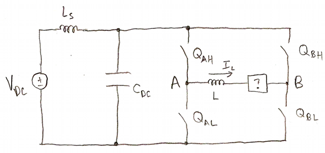
Here we have a typical H-bridge with an inductive load. (Mmmmm ahhh! It's good to draw by hand every once in a while!) There are four power switches: QAH and QAL connecting node A to the DC link, and QBH and QBL connecting node B to the DC link. The load is connected between nodes A and B, and here is represented by an inductive load in series with something else. We don't really care what the something else is, as long as we've pulled out the series inductance L.
The H-bridge is called an H-bridge because it looks like the letter H. (And if you don't see it, move your mouse over the image.) The DC link is called the DC link because it's supposed to be a DC voltage. The usual methodology here is to group the power switches into two half-bridges, one for each of nodes A and B, and pretend that the half-bridges act like switching multipliers.
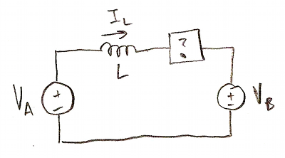
The voltage on node A is equal to VDC for some fraction of the time DA, and is equal to 0 for the rest of the time, so we can treat node A like a voltage source VA equal to DAVDC. Similarly, node B is like a voltage source VB equal to DBVDC. And therefore the voltage across the load is just VAB=(DA - DB)VDC. From here on, proper control over the load voltage and current uses standard control systems techniques with the Laplace transform domain and Z-transform domain.
Whoa! That sidesteps a number of important issues:
- non-ideal switch behavior:
- low-frequency voltage drops in the switches
- dynamics of the switches during turn-on and turn-off
- dead time (the delay between turning off QAH and turning on QAL, or between turning off QAL and turning on QAH, so we don't get a short-circuit across the DC link)
- non-ideal passive component behavior:
- series impedance in the DC link voltage source (inductance Ls, for example)
- series impedance in the DC link capacitor
- what the voltages and currents look like during the switching period
We're not going to talk about the first two of these, at least not right now, but we will talk today about what happens to the load current waveform during the switching period.
First, let's have some fun creating some pulse-width modulation waveforms in Python.
import matplotlib.pyplot as plt
import numpy as np
import scipy.integrate

def ramp(t): return t % 1
def sawtooth(t): return 1-abs(2*(t % 1) - 1)

def pwm(t,D,centeralign = False):
  '''generate PWM signals with duty cycle D'''
  return ((sawtooth(t) if centeralign else ramp(t)) <= D) * 1.0

def digitalplotter(t,*signals):
  '''return a plotting function that takes an axis and plots
digital signals (or other signals in the 0-1 range)'''
  def f(ax):
    n = len(signals)
    for (i,sig) in enumerate(signals):
      ofs = (n-1-i)*1.1
      plotargs = []
      for y in sig[1:]:
        if isinstance(y,basestring):
          plotargs += [y]
        else:
          plotargs += [t,y+ofs]
      ax.plot(*plotargs)
    ax.set_yticks((n-1-np.arange(n))*1.1+0.55)
    ax.set_yticklabels([sig[0] for sig in signals])
    ax.set_ylim(-0.1,n*1.1)
  return f
t = np.arange(0,4,0.0005)
sigA = ('A',pwm(t,0.2,centeralign=True))
sigB = ('B',pwm(t,0.5,centeralign=False))
sigC = ('C',pwm(t,0.9,centeralign=False))

fig = plt.figure()
ax = fig.add_subplot(1,1,1)
digitalplotter(t,
  sigA+(sawtooth(t),'k:'),
  sigB+(ramp(t),'k:'),
  sigC+(ramp(t),'k:'))(ax)
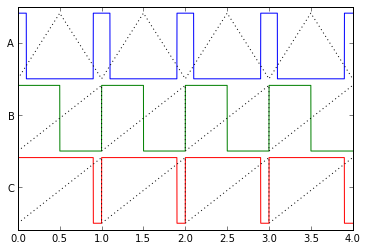
See, that wasn't so hard.
Now we need to think a bit. What voltage really appears across the load? Well, it is Va - Vb, but here we're going to use functions of time rather than DC values. For now, let's ignore the DC link voltage; just assume it's 1.0 volt, so we can look at the raw PWM signals. Also, note that our PWM period is 1.0 rather than 50 μsec or 100μsec. This is called normalizing the equations, and we'll add back these factors of DC link voltage and PWM period later.
pwmA = pwm(t,0.5,centeralign=False)
pwmB = pwm(t,0.2,centeralign=False)

fig = plt.figure()
ax = fig.add_subplot(1,1,1)
digitalplotter(t,
  ('pwmA',pwmA),
  ('pwmB',pwmB),
  ('pwmA-pwmB',pwmA-pwmB))(ax)
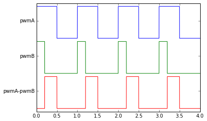
There, the difference between two PWM signals is just a signal that goes between either 0 and 1, or -1 and 0, or -1 and 1, depending on the timing between the signals.
Ripple current
How can we figure out what the current looks like, if we don't know what's in the '?' box of the inductive load?
Here's the trick: as long as the circuit's dominant electrical time constant is long compared to the PWM period, we can confine our interest to high frequency content of the load current. The electrical time constant is approximately L/R, where R is the series resistance of the load; it's exact if there are no other load impedances. If you have R = 0.2 ohm and L = 100 μH, that gives you a time constant of 500 μs, which is quite a bit longer than the usual PWM periods of 50 μs or 100 μs (corresponding to 20 kHz and 10 kHz). For typical motors, the electrical time constant is in the 200 μs - 20 ms range. Other power electronic loads (transformers, etc.) may have lower time constants.
The other part of the trick is that if the electrical time constant is not long compared to the PWM period, we are probably not switching at a high enough frequency. That's because the dynamics of the load current are so fast that we can't ignore what happens in the timescale of pulse-width modulation, and any control system will have to be more complicated.
So in many cases, the frequency content of the load current can be nicely segregated into disjoint pieces: the high-frequency content of ripple current, and the low-frequency content of whatever's in the '?' box. Stated another way:
The ripple current of the load is determined by the content of a PWM waveform at harmonics of the PWM frequency. The average-value model current of the load is determined by the content of a PWM waveform below the PWM frequency. Average-value models are commonly used to design control systems in power electronics, and they assume that the PWM frequency components of the load voltages are absent, and the voltage on node A is equal to DA(t) × VDC where DA(t) is the input to the PWM generator.
So what's the high-frequency content of a PWM waveform? It's just the PWM waveform minus its average value. We can simulate this in Python, too:
def extendrange(ra,rb):
  '''return a tuple (x1,x2) representing the interval from x1 to x2,
given two input ranges of the same form, or None (representing no input).'''
  if ra is None:
    return rb
  elif rb is None:
    return ra
  else:
    return (min(ra[0],rb[0]),max(ra[1],rb[1]))

def createLimits(margin, *args):
    '''add proportional margin to an interval:
createLimits(0.1, (1,3),(2,4),(0,2)) calculates the maximum extent
of the ranges provided, in this case (0,4), and adds another 0.1 (10%)
to the extent symmetrically, thus returning (-0.2, 4.2).'''
    r = None
    for x in args:
        r = extendrange(r, (np.min(x),np.max(x)))
    rmargin = (r[1]-r[0])*margin/2.0
    return (r[0]-rmargin,r[1]+rmargin)

def calcripple(t,y):
    ''' calculate ripple current by integrating the input,
then adjusting it by a linear function to put both endpoints
at the same value. The slope of the linear function is the
mean value of the input; the offset is chosen to make the mean value
of the output ripple current = 0.'''
    T = t[-1]-t[0]
    yint0 = np.append([0],scipy.integrate.cumtrapz(y,t))
    # cumtrapz produces a vector of length N-1
    # so we need to add one element back in at the beginning
    meanval0 = yint0[-1]/T
    yint1 = yint0 - (t-t[0])*meanval0
    meanval1 = scipy.integrate.trapz(yint1,t)/T
    return yint1 - meanval1

def showripple(fig,t,Va,Vb,titlestring):
    '''plot ripple current as well as phase duty cycles and load voltage'''
    axlist = []
    Iab = calcripple(t,Va-Vb)
    margin = 0.1
    ax = fig.add_subplot(3,1,1)
    digitalplotter(t,('Va',Va),('Vb',Vb))(ax)
    ax.set_ylabel('Phase duty cycles')
    axlist.append(ax)

    ax = fig.add_subplot(3,1,2)
    ax.plot(t,Va-Vb)
    ax.set_ylim(createLimits(margin,Va-Vb))
    ax.set_ylabel('Load voltage')
    axlist.append(ax)

    ax = fig.add_subplot(3,1,3)
    ax.plot(t,Iab)
    ax.set_ylim(createLimits(margin,Iab))
    ax.set_ylabel('Ripple current')
    axlist.append(ax)

    fig.suptitle(titlestring, fontsize=16)

    # annotate with peak values
    tlim = [min(t),max(t)]
    tannot0 = tlim[0] + (tlim[1]-tlim[0])*0.5
    tannot1 = tlim[0] + (tlim[1]-tlim[0])*0.6
    for y in [min(Iab),max(Iab)]:
      ax.plot(tlim,[y]*2,'k:')
      # see:
# http://matplotlib.org/api/axes_api.html#matplotlib.axes.Axes.annotate
      ax.annotate('%.5f' % y, xy=(tannot0,y), xytext=(tannot1,y*0.3),
        bbox=dict(boxstyle="round", fc="0.9"),
        arrowprops=dict(arrowstyle="->",
          connectionstyle="arc,angleA=0,armA=20,angleB=%d,armB=15,rad=7"
             % (-90 if y > 0 else 90))
      )
    return axlist

def showpwmripple(fig,t,Da,Db,centeralign=False,titlestring=''):
    return showripple(fig,t,
               pwm(t,Da,centeralign),
               pwm(t,Db,centeralign),
               titlestring='%s-aligned pwm, $D_a$=%.3f, $D_b$=%.3f' %
                 ('Center' if centeralign else 'Edge', Da, Db))
fig = plt.figure(figsize=(8, 6), dpi=80)
showpwmripple(fig,t,0.4,0.2,centeralign=False);
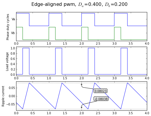
fig = plt.figure(figsize=(8, 6), dpi=80)
showpwmripple(fig,t,0.6,0.2,centeralign=True);
If we want to know what the ripple looks like in general, and not just for a specific case, we have to do some algebra. (Luckily, if you're clumsy like me you can use Python's sympy library to help.)
The edge-aligned case is fairly easy to analyze. Let's say the PWM period is T, and let's define D = Da - Db. If D > 0, then the load voltage is Vdc for a period of time DT and 0 otherwise. If D < 0, then the load voltage is -Vdc for a period of time -DT and 0 otherwise.
This means the average load voltage is DVdc, whether D > 0 or not.
Let's just consider the D > 0 case for now.
Remember: the average or low-frequency load voltage appears across the noninductive components of the load, and the high-frequency load voltage appears across the load inductance.
This means that during the time interval DT, when the load voltage is Vdc, the voltage across the load inductance is Vdc - (average load voltage) = Vdc - DVdc = (1-D)Vdc, and the inductor current increases by \( \Delta I = \int V/L \ dt = \int_0^{DT} (1-D)V_{dc}/L \ dt = D(1-D)V_{dc}T/L \).
During the rest of the PWM period, an interval (1-D)T, when the load voltage is 0, the voltage across the load inductance is 0 - (average load voltage) = 0 - DVdc = -DVdc, and the inductor current increases by \( \Delta I = \int V/L \ dt = \int_{DT}^{T} -DV_{dc}/L \ dt = -(1-D)DV_{dc}T/L \).
Note that the increases in inductor currents have equal amplitudes and opposite signs; the net increase in inductor current over a PWM period, due to PWM voltage harmonics, is exactly 0. Changes in average inductor current are created by low-frequency components of load voltage, where the applied voltage is not equal to the load's DC voltage (whether it's I*R from resistive voltage drops, or something else from motor back-emf).
The last part of this equation, VdcT/L, appears in any ripple current calculation, so let's define a normalized ripple current IR0 = VdcT/L, in which case the peak-to-peak ripple current is just D(1-D)IR0. (Alternatively, the zero-to-peak ripple current is half of that, or D(1-D)IR0/2.) If we go through the same analysis for D<0, we'll end up with a peak-to-peak ripple current of \( |D|(1-|D|)I_{R0} \) handling both cases. (zero-to-peak ripple current = \( |D|(1-|D|)I_{R0}/2 \))
The maximum ripple current is IR0/4 peak-to-peak, when D = ±0.5. Here's what the ripple current looks like as a function of D:
D = np.arange(-1,1,0.005)
plt.plot(D,abs(D)*(1-abs(D)))
plt.xlabel('net duty cycle $D = D_a - D_b$',fontsize=16)
plt.ylabel('ripple current / $I_{R0}$',fontsize=16)
Let's double check this point of maximum ripple current, just to make sure it makes sense. With Da = 0.6 and Db = 0.1, we have D = Da-Db = 0.5 and the peak-to-peak current normalized to IR0 should be 0.25 (namely from -0.125 to +0.125):
fig = plt.figure(figsize=(8, 6), dpi=80)
showpwmripple(fig,t,0.6,0.1,centeralign=False);
That's pretty close! The error here is numerical and we can improve it by using a smaller timestep:
tfine = np.arange(0,4,0.0001)
fig = plt.figure(figsize=(8, 6), dpi=80)
showpwmripple(fig,tfine,0.6,0.1,centeralign=False);

The center-aligned case is a little more difficult to analyze, because there are 4 time intervals per PWM period rather than 2.
If you don't like yucky algebra, skip ahead to the center-aligned results. I don't usually like to put algebraic derivations in blog posts, since I hated sitting through college classes waiting for professors to finish writing long equations on the blackboard, but here I will, since the algebra's not so bad, and it'll give you a sense of how to understand the results if you want, as well as how to use sympy as a tool for assisting with this kind of task.
For Da > Db, these are the four time intervals [A]-[D]:
- [A]: (1-Da)T when the load voltage is zero
- [B]: (Da-Db)T/2 when the load voltage is VDC
- [C]: (Db)T when the load voltage is zero
- [D]: (Da-Db)T/2 when the load voltage is VDC
fig = plt.figure(figsize=(8, 6), dpi=80)
Da,Db = 0.6, 0.1
intcodes = 'ABCD'
axlist = showpwmripple(fig,t,Da,Db,centeralign=True)
for (i,tcenter) in enumerate([0.5, 1-(Da+Db)/4, 1, 1+(Da+Db)/4]):
    y = (i/2) * 1.1 + 0.55
    intcode = '[%s]' % intcodes[i]
    axlist[0].annotate(intcode,xy=(tcenter,y),
        horizontalalignment='center',
        verticalalignment='center')
    axlist[2].annotate(intcode,xy=(tcenter,0.05),
        horizontalalignment='center',
        verticalalignment='center')
Let's focus on one period and look at the results. The average load voltage is still DVDC = (Da-Db)VDC. If we go through a similar type of analysis as the edge-aligned case, let's look at the values of the normalized inductor current (factoring out a VDCT/L) at some strategically-chosen times:
def show1period(Da,Db):
  t1period = np.arange(-0.5,1.5,0.001)
  pwmA = pwm(t1period,Da,centeralign=True)
  pwmB = pwm(t1period,Db,centeralign=True)
  fig = plt.figure()
  ax = fig.add_subplot(1,1,1)
  Ir = calcripple(t1period,pwmA-pwmB)
  ax.plot(t1period,Ir)
  ax.set_xlim(-0.1,1.1)
  ax.set_ylim(min(Ir)*1.2,max(Ir)*1.2)
  # now annotate
  (D1,D2,V) = (Db,Da,1) if Da > Db else (Da,Db,-1)
  tpts = np.array([0, D1/2, D2/2, 0.5, 1-(D2/2), 1-(D1/2), 1])
  dtpts = np.append([0],np.diff(tpts))
  vpts = np.array([0, 0, V, 0, 0, V, 0]) - (Da-Db)
  ypts = np.cumsum(vpts*dtpts)
  ax.plot(tpts,ypts,'.',markersize=8)
  for i in range(7):
    ax.annotate('$t_%d$' % i,xy=(tpts[i]+0.01,ypts[i]), fontsize=16)

show1period(0.6,0.1)
show1period(0.9,0.8)

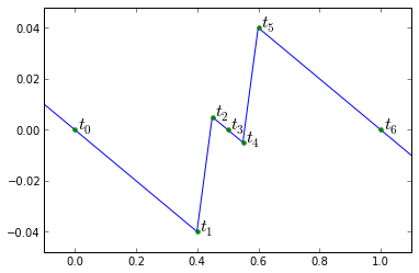
For D = Da - Db > 0, here's algebraic equations for the ripple current values at these points t[0] - t[6]:
| t/T | I/IR0 |
|---|---|
| t[0] = 0 | I[0] = 0 |
| t[1] = Db/2 | I[1] = I[0] + (t[1]-t[0])*(0-D) = -D*Db/2 |
| t[2] = Da/2 | I[2] = I[1] + (t[2]-t[1])*(1-D) = -D*Db/2 + (Da-Db)*(1-D)/2 |
| t[3] = 0.5 | I[3] = I[2] + (t[3]-t[2])*(0-D) = -D*Db/2 + (Da-Db)*(1-D)/2 + (1-Da)*(0-D)/2 |
| t[4] = 1-Da/2 | I[4] = I[3] + (t[4]-t[3])*(0-D) = yucky algebra |
| t[5] = 1-Db/2 | I[5] = I[4] + (t[5]-t[4])*(1-D) = yucky algebra |
| t[6] = 1 | I[6] = I[5] + (t[6]-t[5])*(0-D) = yucky algebra |
The algebra is starting to get a bit yucky, so let's simplify this with sympy. The algebra trick we'll use is to rewrite Da and Db in terms of their differential-mode component D and common-mode component D0:
import sympy
%load_ext sympy.interactive.ipythonprinting
D, D0 = sympy.symbols("D D_0")
Da =  D/2 + D0
Db = -D/2 + D0
# now let's verify that we've defined D and D0 properly:
display('Da-Db=',Da-Db)
display('(Da+Db)/2=',(Da+Db)/2)
Da-Db=
(Da+Db)/2=
# average voltage at the load = D
I = [0,0,0,0,0,0,0]
I[1] = I[0] + Db/2*(0-D)
I[2] = I[1] + (Da-Db)/2*(1-D)
I[3] = I[2] + (1-Da)/2*(0-D)
I[4] = I[3] + (1-Da)/2*(0-D)
I[5] = I[4] + (Da-Db)/2*(1-D)
I[6] = I[5] + Db/2*(0-D)

# let's use pandas to display as a table
import pandas as pd
itable1 = pd.DataFrame([sympy.simplify(Ik) for Ik in I],
             index=['I[%d]' % d for d in range(7)])
itable1
| 0 | |
|---|---|
| I[0] | 0 |
| I[1] | D*(D - 2*D_0)/4 |
| I[2] | D*(-D - 2*D_0 + 2)/4 |
| I[3] | 0 |
| I[4] | D*(D + 2*D_0 - 2)/4 |
| I[5] | D*(-D + 2*D_0)/4 |
| I[6] | 0 |
It's always good to see 0 values when you're simplifying algebra. Also note that I[1] = -I[5] and I[2] = -I[4]. If we were to repeat this exercise for D < 0 (Da < Db), we'd get:
# average voltage at the load = D;
# load voltage alternates between 0 and -1
I = [0,0,0,0,0,0,0]
I[1] = I[0] + Da/2*(0-D)
I[2] = I[1] + (Db-Da)/2*(-1-D)
I[3] = I[2] + (1-Db)/2*(0-D)
I[4] = I[3] + (1-Db)/2*(0-D)
I[5] = I[4] + (Db-Da)/2*(-1-D)
I[6] = I[5] + Da/2*(0-D)
itable2 = pd.DataFrame([sympy.simplify(Ik) for Ik in I],
                index=['I[%d]' % d for d in range(7)])
itable2
| 0 | |
|---|---|
| I[0] | 0 |
| I[1] | D*(-D - 2*D_0)/4 |
| I[2] | D*(D - 2*D_0 + 2)/4 |
| I[3] | 0 |
| I[4] | D*(-D + 2*D_0 - 2)/4 |
| I[5] | D*(D + 2*D_0)/4 |
| I[6] | 0 |
The forms are the same, and we can generalize to this:
I[0] = I[3] = I[6] = 0
I[1] = -I[5] = D*(abs(D) - 2*D0)/4
I[2] = -I[4] = D*(2-abs(D) - 2*D0)/4
The maximum amplitude of ripple current is just the maximum amplitude of I[1] or I[2]:
I[peak] = abs(D)*max(abs(abs(D) - 2*D0), abs(2 - abs(D) - 2*D0))/4
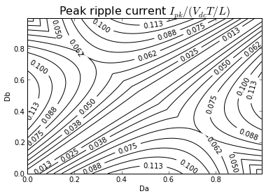
We can plot this in a contour plot in Python:
Da_vector = np.arange(0,1,0.005)
Db_vector = np.arange(0,1,0.005)
Da, Db = np.meshgrid(Da_vector, Db_vector)
D = Da-Db
D0 = (Da+Db)/2
Ipk = abs(D)*np.maximum(abs(abs(D)-2*D0),abs(2-abs(D)-2*D0))/4
cs = plt.contour(Da,Db,Ipk,numpy.arange(0,0.125,0.0125),colors='black')
plt.clabel(cs)
plt.xlabel('Da')
plt.ylabel('Db')
plt.title('Peak ripple current $I_{pk}/(V_{dc}T/L)$',fontsize=16)
Text(0.5,1,'Peak ripple current $I_{pk}/(V_{dc}T/L)$')
It may be a bit more insightful to make a contour plot relative to the common-mode and differential-mode duty cycles:
cs = plt.contour(D,D0,Ipk,numpy.arange(0,0.125,0.0125),
             colors='black')
plt.clabel(cs)
plt.xlabel('D = Da - Db')
plt.xticks(np.arange(-1,1.25,0.25))
plt.yticks(np.arange(0,1.1,0.1))
plt.ylabel('common-mode duty cycle D0')
plt.title('Peak ripple current $I_{pk}/(V_{dc}T/L)$',
  fontsize=16)
Text(0.5,1,'Peak ripple current $I_{pk}/(V_{dc}T/L)$')
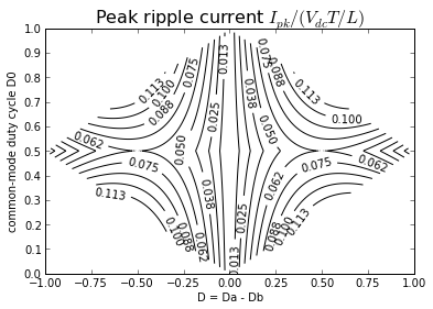
Why is this insightful? Because the minimum amplitude ripple occurs when we keep the common-mode duty cycle equal to 0.5! In this case, we pick our differential duty cycle D, and set Da = (1 + D)/2 and Db = (1 - D)/2.
Not only do we get ripple current of minimum amplitude for a given differential duty cycle D, but the irregular-looking waveform for ripple current disappears, and we're left with a straightforward sawtooth at twice the PWM frequency:
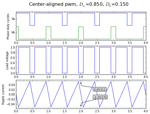
fig = plt.figure(figsize=(8, 6), dpi=80)
Da,Db = 0.25, 0.75
axlist = showpwmripple(fig,t,Da,Db,centeralign=True)
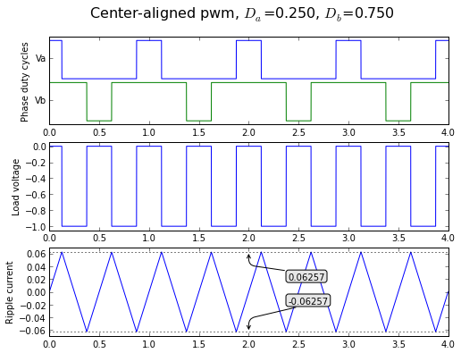
fig = plt.figure(figsize=(8, 6), dpi=80)
Da,Db = 0.85, 0.15
axlist = showpwmripple(fig,t,Da,Db,centeralign=True)
If we take that somewhat ugly equation for peak ripple current:
I[peak] = abs(D) * max(abs(abs(D) - 2*D0),abs(2 - abs(D) - 2*D0))/4
and substitute D0 = 0.5, we get:
I[peak] = abs(D) * max(abs(abs(D) - 1),abs(2 - abs(D) - 1))/4 = abs(D) * max(abs(abs(D) - 1),abs(1 - abs(D)))/4
But abs(abs(D) - 1) and abs(1 - abs(D)) are both equal to 1 - abs(D), so we have
I[peak] = |D| * (1-|D|) / 4.
This is exactly 1/2 the ripple current of the edge-aligned case! We get half the ripple at twice the frequency!
TL;DR:
Center-aligned PWM is Better Than Edge-aligned PWM
If you take away only two things from this article, and forget everything else, they should be:
- center-aligned PWM is better than edge-aligned PWM
- when using center-aligned PWM in an H-bridge, center your A and B phase around 0.5: Da = (1+D)/2, Db = (1-D)/2
If you follow these two simple rules, you will double the ripple frequency content, and reduce the ripple amplitude by a factor of 2, compare to edge-aligned PWM.
There are valid reasons to deviate from these rules significantly, but they're rare. If you have a system with very high switching losses (where you may not want to keep switching all 4 switches on and off during a PWM period), it may be important to create switching waveforms that allow you to keep some of the transistors either open or closed during the entire PWM cycle. (You can do this with 3 out of the 4 switches, at the cost of higher ripple current, and diode conduction rather than transistor conduction in one of the switches.) This removes switching losses in those transistors.
A more common situation is a system with bootstrap capacitor gate drives, where the upper transistors can't be turned on at 100% duty cycle, or the bootstrap capacitor will deplete its charge. The maximum duty cycle you can reach depends on the detailed characteristics of the gate drive circuitry, but typically is in the 90-98% range. (If someone working on a gate drive design came to me and said they can only reach 90% duty cycle on the upper transistors, I'd ask why, and send them back to the drawing board to do better.) The lower transistors, on the other hand, can be kept on at 100% duty cycle. So this creates a slight asymmetry, and the best solution is to come as close as you can to the ideal case, which means to reduce the common-mode duty cycle slightly at large modulation indices. Maybe that wasn't clear, so here's a concrete example:
Suppose you have a system with an H-bridge, but it has gate drive circuitry which limits your effective duty cycle on each half-bridge between 0 and 90%. And you're working with a control systems guru, who wants to see a particular duty cycle D applied across the load. It's your job to pick half-bridge duty cycles Da and Db, so here's what you might run into:
| D | Da (ideally) | Db (ideally) | Ipk-pk (ideally) | Da | Db | D0 = (Da+Db)/2 | Ipk-pk |
|---|---|---|---|---|---|---|---|
| 0 | 50% | 50% | 0 | 50% | 50% | 50% | 0 |
| 20% | 60% | 40% | 0.08 IR0 | 60% | 40% | 50% | 0.08 IR0 |
| 40% | 70% | 30% | 0.12 IR0 | 70% | 30% | 50% | 0.12 IR0 |
| 60% | 80% | 20% | 0.12 IR0 | 80% | 20% | 50% | 0.12 IR0 |
| 80% | 90% | 10% | 0.08 IR0 | 90% | 10% | 50% | 0.08 IR0 |
| 84% | 92% | 8% | 0.0672 IR0 | 90% | 6% | 48% | 0.084 IR0 |
| 88% | 94% | 6% | 0.0528 IR0 | 90% | 2% | 46% | 0.088 IR0 |
| 90% | 95% | 5% | 0.045 IR0 | 90% | 0% | 45% | 0.09 IR0 |
| 92% | 96% | 4% | 0.0368 IR0 | 90% | 0% | 45% | 0.09 IR0 |
| 96% | 98% | 2% | 0.0192 IR0 | 90% | 0% | 45% | 0.09 IR0 |
| 100% | 100% | 0% | 0 | 90% | 0% | 45% | 0.09 IR0 |
The ideal case isn't achievable in real life; you can't get an output duty cycle across the load of more than 90%, and once you reach 80% output duty cycle, you have to move the common-mode duty downward slightly to ensure that the upper transistors aren't on more than 90% of the time. In this case, ripple current increases slightly at high load voltages.
RMS and harmonic components of ripple current
OK, we have the zero-to-peak ripple current formula for center-aligned PWM in an H-bridge, with duty cycles centered around 50%:
$$D_a = \frac{1+D}{2}$$
$$D_b = \frac{1-D}{2}$$
$$I_{pk} = \frac{|D| (1-|D|)}{4} I_{R0}$$
where $$I_{R0} = \frac{V_{DC}T}{L}$$
but what about RMS and the harmonic content of the ripple current waveform?
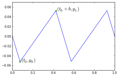
Root-mean-square current (RMS)
Our ripple current waveform is piecewise linear. For a time period = DT/2, the ripple current rises linearly from -Ipk to +Ipk, and then for a time period = (1-D)T/2, the ripple current falls linearly from +Ipk to -Ipk.
RMS current is defined as the square root of the mean value of the squared current. Let's figure out how we can analyze this:
t2 = np.arange(0,1,0.001)
D = 0.7
t0 = (1-D)/4
t1 = (1+D)/4
y1 = abs(D)*abs(1-D)/4
Vload = (pwm(t2,(1.0+D)/2,centeralign=True)
        -pwm(t2,(1.0-D)/2,centeralign=True))
I = calcripple(t2,Vload)
plt.plot(t2,I)
plt.ylim(-0.07,0.07)
plt.plot([t0,t1],[-y1,y1],'.',markersize=8)
plt.annotate('$(t_0,y_0)$',xy=(t0+0.01,-y1),fontsize=16)
plt.annotate('$(t_0+h,y_1)$',xy=(t1+0.01,y1),fontsize=16)
Annotation(0.435,0.0525,'$(t_0+h,y_1)$')
t,t0,y0,y1,h = sympy.symbols('t t0 y0 y1 h')
m = (y1-y0)/h
y = m*(t-t0)+y0
integral_ysquared = sympy.integrate(y**2,(t,t0,t0+h))
display('integral of y^2 = ',sympy.simplify(integral_ysquared))
integral of y^2 =
What did we just do here? We defined y as a linear function of t, where \( y\vert_{t=t0} = y_0 \), and \( y\vert_{t=t0+h} = y1 \). The slope is just \( m=\frac{y_1-y_0}{h} \). The integral of y2 over this range is a very simple expression.
How does this help us with the RMS of piecewise linear waveforms? For any function \( f(t) \) defined over an interval between t = T0 and t = T1, the root-mean-square of \( f(t) \) over that interval is defined as:
$$RMS(f(t),T_0,T_1) = \sqrt{\frac{\int_{T_0}^{T_1} f(t)^2 dt}{T_1-T_0}}$$
So let's apply this to our sawtooth with amplitude Ipk.
The integral of Iripple^2 is equal to \( \frac{1}{3} * (DT/2) * ((-I_{pk})^2 + (-I_{pk})*(I_{pk}) + (I_{pk})^2) \) for the first time period, DT/2, and then \( \frac{1}{3} * ((1-D)T/2) * ((I_{pk})^2 + (I_{pk}) * (-I_{pk}) + (-I_{pk})^2) \) for the rest of the time period, (1-D) * T/2.
Then we have to take the average over the time T/2, and the square root:
Too much math for you? Let sympy do the work:
Ipk,D,T = sympy.symbols('I_{pk} D T')
def f3(y0,y1,h):
    return h*(y0*y0 + y0*y1 + y1*y1)/3
integral_squared_ripple = (f3(-Ipk,Ipk,D*T/2) + f3(Ipk,-Ipk,(1-D)*T/2))
sympy.simplify(integral_squared_ripple/(T/2))
If we take the square root of this, sympy won't oblige, because it doesn't know that Ipk is non-negative. But we do, so the RMS value of the ripple current is just \( I_{pk}/\sqrt{3} \). Substitute in our equation for Ipk as a function of D, and we get:
$$I_{ripple,rms} = I_{R0}\frac{|D|(1-|D|)}{4\sqrt{3}}$$
Ripple harmonic amplitudes
Need to perform Fourier analysis? Then sympy can help:
def piecewiseHarmonic(flist,tlist,k,T=1,t=None):
    ''' calculates piecewise integration of the
kth harmonic of a given function

flist is a list of N functions
tlist is a list of N+1 points in time
piecewiseHarmonic() calculates the sum of the
  integral of flist[i]*exp(2j*pi*k*t/T)
  between t=tlist[i] and tlist[i+1]
  iterating over i = 0:N-1
'''
    S = 0
    t = sympy.symbols('t') if t is None else t
    pi = sympy.pi
    for (i,f) in enumerate(flist):
        dt_range = (t,tlist[i],tlist[i+1])
        S += 2*sympy.integrate(f*sympy.cos(2*pi*k*t/T),dt_range)/T
        S += 2j*sympy.integrate(f*sympy.sin(2*pi*k*t/T),dt_range)/T
    return sympy.simplify(S)

t=sympy.symbols('t')
def cosk(k):
    return sympy.cos(2*sympy.pi*k*t)
def sink(k):
    return sympy.sin(2*sympy.pi*k*t)

display(piecewiseHarmonic([cosk(3)],[0,1],3))
display(piecewiseHarmonic([cosk(3)],[0,1],4))
display(piecewiseHarmonic([sink(3)],[0,1],3))
display(piecewiseHarmonic([sink(3)],[0,1],4))
To analyze the harmonics of a sawtooth, we need to define the sawtooth in terms of piecewise linear functions:
def sawtooth_up(D,t):
    return (1-D)*(4*t-1)/4

def sawtooth_down(D,t):
    return (-D)*t

D = 0.7
t_down = numpy.arange(-(1-D)/2,(1-D)/2,0.001)
t_up = numpy.arange((1-D)/2,(1+D)/2,0.001)
plt.plot(t_down/2,sawtooth_down(D,t_down/2),
         t_up/2,sawtooth_up(D,t_up/2))
plt.grid('on')
D,t = sympy.symbols('D t')
for k in range(6):
    display('harmonic #%d' % k,piecewiseHarmonic(
            [sawtooth_down(D,t/2),
             sawtooth_up(D,t/2)],
            [-(1-D)/2,(1-D)/2,(1+D)/2],k))
harmonic #0
harmonic #1
harmonic #2
harmonic #3
harmonic #4
harmonic #5
If you try to get sympy to handle this for general integers k, it doesn't seem to figure out a simplified answer, so I just printed out the first few terms for fixed integers k.
The "i" in the answer tells us that the coefficients are pure imaginary and therefore the Fourier series is only sine terms, not cosine terms. The general form of these harmonics has a real part of 0 and an imaginary part of $$A_k = \frac{(-1)^k \sin k\pi D}{k^2\pi^2}$$
At first I thought I must have made a mistake; sawtooth waveforms should have only odd harmonics, right? But let's plot the results, and you'll see that they're right on the money; the even harmonics only disappear when D = 0.5.
def sawtoothApprox(D,kmax,printHarmonics=False):
    pi = numpy.pi
    def f(t):
        S = 0
        for k in range(1,kmax+1):
            a_k = (-1)**k / 2.0 / k / k
            A_k = sin(k*pi*D)*a_k/pi/pi
            if printHarmonics:
                print 'for k=%d, a_k=%9.6f, A_k=%9.6f' % (k,a_k,A_k)
            S += A_k*sin(2*pi*k*t)
        return S
    return f

t2 = np.arange(0,1,0.001)
D = 0.7
Vload = (pwm(t2,(1.0+D)/2,centeralign=True)
       - pwm(t2,(1.0-D)/2,centeralign=True))
I = calcripple(t2,Vload)
Iapprox = sawtoothApprox(D,6,printHarmonics=True)(2*t2)
# show exact sawtooth, approximation of 1st 6 harmonics,
# and then the approximation error
plt.plot(t2,I,t2,Iapprox,t2,(I-Iapprox),':k')
for k=1, a_k=-0.500000, A_k=-0.040985
for k=2, a_k= 0.125000, A_k=-0.012045
for k=3, a_k=-0.055556, A_k=-0.001739
for k=4, a_k= 0.031250, A_k= 0.001861
for k=5, a_k=-0.020000, A_k= 0.002026
for k=6, a_k= 0.013889, A_k= 0.000827
[Line2D(_line0), Line2D(_line1), Line2D(_line2)]
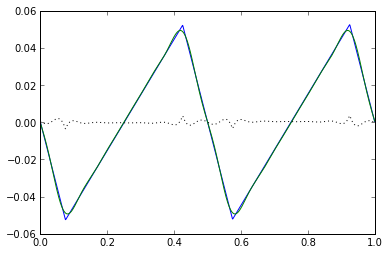
In a nutshell: the bulk of the energy in a sawtooth waveform is in the 1st and 2nd harmonic. (For center-aligned PWM, this translates into the 2nd and 4th harmonic of the PWM frequency.)
RMS of That Ugly Suboptimal Center-Aligned PWM
The above analysis is for PWM which creates a simple sawtooth waveform, which is the case for edge-aligned PWM, and for center-aligned PWM with the common-mode duty cycle fixed at 50%.
For center-aligned PWM with common-mode duty cycle other than 50%, the ripple current waveform is "uglier". Remember the waveform shown below?
show1period(0.6,0.1)
We used sympy and some "human-directed" algebra to figure out the currents at each of the time instants \( t_0 \) - \( t_6 \). Here it is again in a more concise form:
$$I_L(t_0) = I_L(t_3) = I_L(t_6) = 0$$
$$I_L(t_1) = -I_L(t_5) = D \times (|D| - 2D_0)/4$$
$$I_L(t_2) = -I_L(t_4) = D \times (2-|D| - 2D_0)/4$$
$$D = D_a - D_b, D_0 = (D_a + D_b) / 2 $$
$$I_{pk} = \max(|I_L(t_1)|,|I_L(t_2)|)$$
Calculating RMS of this waveform is a little more difficult than in the other cases, but it's not horrible. There are seven points here, but \( t_0, t_3, t_6 \) are all in the middle of line segments so we're really left with four intervals of linear segments:
- \( [t_1, t_2] \) with length \( |D|T/2 \)
- \( [t_2, t_4] \) with length \( 1-\max(D_a,D_b) = (1-D_0-|D|/2)T \)
- \( [t_4, t_5] \) with length \( |D|T/2 \)
- \( [t_5, t_1] \) with length \( \min(D_a,D_b) = (D_0-|D|/2)T \).
And that's enough information to calculate RMS current:
D,D0,D0dev,T = sympy.symbols('D D_0 D_{0dev} T')
def f3(y0,y1,h):
    return h*(y0*y0 + y0*y1 + y1*y1)/3
I1 = D*(abs(D)-2*D0)/4
I2 = D*(2-abs(D)-2*D0)/4
integral_squared_ripple = (
   f3(I1,I2,abs(D)/2*T)
 + f3(I2,-I2,(1-D0-abs(D)/2)*T)
 + f3(-I2,-I1,abs(D)/2*T)
 + f3(-I1,I1,(D0-abs(D)/2))*T)
mean_squared_ripple = sympy.simplify(integral_squared_ripple/T)
mean_squared_ripple
We have to play a little trick on sympy to get it to clean this up a little bit. The "ugliness" of this waveform disappears at \( D_0 = \tfrac{1}{2} \), so let's substitute \( D_{0dev} = D_0 - \tfrac{1}{2} \), simplify, and substitute back:
Int1 = sympy.Integer(1)
msr2 = sympy.simplify(mean_squared_ripple.subs(D0, D0dev + Int1/2)).subs(D0dev,D0-Int1/2)
display('mean squared ripple = ',msr2)
mean squared ripple =
Looks like sympy still needs some help, so let's finish the simplification by hand. The easiest thing here is that \( |D|^2 - 2|D| + 1 = (1-|D|)^2 \). Also, remember that we are looking for RMS ripple, which is the square root of mean squared ripple:
$$RMS(I_L) = \frac{|D|\sqrt{12(D_0-\tfrac{1}{2})^2 + (1-|D|)^2}}{4\sqrt{3}}$$
For the simplified case where \( D_0 = \tfrac{1}{2} \), the RMS equation simplifies to the same expression we obtained earlier.
While we're at it, let's take a whack at simplifying the peak ripple current. It looks like sympy can't help us get there, but we can spot check my algebra at a few values. Here's what I get when I simplify things:
$$|I_L(t_1)| = \frac{|D|}{4} |1-|D| + 2(D_0 - \tfrac{1}{2})|$$ $$|I_L(t_2)| = \frac{|D|}{4} |1-|D| - 2(D_0 - \tfrac{1}{2})|$$ $$\max(|I_L(t_1)|,|I_L(t_2)|) = \frac{|D|(1-|D|)}{4} + \frac{|D| |D_0 - \tfrac{1}{2}|}{2}$$
Let's verify whether this is correct:
def check_jasons_algebra(D,D0):
  # here's what we know for certain
  I1 = D*(abs(D)-2*D0)/4
  I2 = D*(2-abs(D)-2*D0)/4
  # here's what I got with algebra by hand
  Ipk = abs(D)*(1-abs(D))/4 + abs(D)*abs(D0-0.5)/2
  print("D=%f,D0=%f,I1=%f,I2=%f" % (D,D0,I1,I2))
  print("max(abs(I1),abs(I2))=%f, Jason's calc=%f"
    % (max(abs(I1),abs(I2)), Ipk))

for (D,D0) in (
      (0.5,0.5),
      (0.5,0.4),
      (0.5,0.6),
      (0.1,0.5),
      (0.1,0.4),
      (0.1,0.6),
      (-0.5,0.5),
      (-0.5,0.4),
      (-0.5,0.6)
      ):
  check_jasons_algebra(D,D0)
D=0.500000,D0=0.500000,I1=-0.062500,I2=0.062500
max(abs(I1),abs(I2))=0.062500, Jason's calc=0.062500
D=0.500000,D0=0.400000,I1=-0.037500,I2=0.087500
max(abs(I1),abs(I2))=0.087500, Jason's calc=0.087500
D=0.500000,D0=0.600000,I1=-0.087500,I2=0.037500
max(abs(I1),abs(I2))=0.087500, Jason's calc=0.087500
D=0.100000,D0=0.500000,I1=-0.022500,I2=0.022500
max(abs(I1),abs(I2))=0.022500, Jason's calc=0.022500
D=0.100000,D0=0.400000,I1=-0.017500,I2=0.027500
max(abs(I1),abs(I2))=0.027500, Jason's calc=0.027500
D=0.100000,D0=0.600000,I1=-0.027500,I2=0.017500
max(abs(I1),abs(I2))=0.027500, Jason's calc=0.027500
D=-0.500000,D0=0.500000,I1=0.062500,I2=-0.062500
max(abs(I1),abs(I2))=0.062500, Jason's calc=0.062500
D=-0.500000,D0=0.400000,I1=0.037500,I2=-0.087500
max(abs(I1),abs(I2))=0.087500, Jason's calc=0.087500
D=-0.500000,D0=0.600000,I1=0.087500,I2=-0.037500
max(abs(I1),abs(I2))=0.087500, Jason's calc=0.087500
Looks good to me!
3-phase PWM
The extension of this type of analysis for 3-phase PWM is more difficult, and the result is more complex. Describing the ripple current in 3-phase PWM is something I may do at work, in the form of a Microchip application note. Watch for it someday, at http://www.microchip.com/motorcontrol.
Summary
Here's a summary of ripple current statistics for H-bridge PWM. Remember, \( D = D_a - D_b \) is the effective load duty cycle, \( D_0 = (D_a + D_b)/2 \) is the common-mode duty cycle, and \( I_{R0} = V_{DC}T/L \) is a reference current that simplifies calculation of these statistics.
Let's also define \( I_R = |D|(1-|D|)I_{R0} \), and \( I_{R2} = 2|D||D_0-\tfrac{1}{2}|I_{R0} \) since they will appear several times in the following table.
| PWM type | Peak to peak ripple | Peak ripple | RMS ripple | fundamental frequency | amplitude of kth harmonic |
|---|---|---|---|---|---|
| edge-aligned | \( I_R \) | \( \frac{1}{2}I_R \) | \( \frac{1}{2\sqrt{3}}I_R \) | \( f_{PWM} = 1/T \) | $$A_k = \frac{(-1)^k \sin k\pi D}{k^2\pi^2} I_{R0}$$ |
| center-aligned (common-mode = 0.5) |
\( \frac{1}{2}I_R \) | \( \frac{1}{4}I_R \) | \( \frac{1}{4\sqrt{3}}I_R \) | \( 2f_{PWM} \) | $$A_k = \frac{(-1)^k \sin k\pi D}{2k^2\pi^2} I_{R0}$$ |
| center-aligned (common-mode ≠ 0.5) |
\( \frac{I_R+I_{R2}}{2} \) | \( \frac{I_R+I_{R2}}{4} \) | \( \frac{|D|\sqrt{12(D_0-\tfrac{1}{2})^2 + (1-|D|)^2}}{4\sqrt{3}}I_{R0} \) | \( f_{PWM} \), but 1st harmonic has low amplitude if D0 is close to 0.5 |
exercise for the reader |
To keep the ripple current minimized, use center-aligned PWM whenever possible, and keep the common-mode duty cycle as close to \( \frac{1}{2} \) as possible, by choosing duty cycles as close as practical to \( D_a = (1+D)/2 \), \( D_b = (1-D)/2 \).
Happy switching!
© 2013 Jason M. Sachs
This post is available in an IPython Notebook at https://bitbucket.org/jason_s/embedded-blog-public
Licensed under the Apache License, Version 2.0 (the "License"); you may not use this file except in compliance with the License. You may obtain a copy of the License at
http://www.apache.org/licenses/LICENSE-2.0
Unless required by applicable law or agreed to in writing, software distributed under the License is distributed on an "AS IS" BASIS, WITHOUT WARRANTIES OR CONDITIONS OF ANY KIND, either express or implied. See the License for the specific language governing permissions and limitations under the License.


- Comments
- Write a Comment Select to add a comment
To post reply to a comment, click on the 'reply' button attached to each comment. To post a new comment (not a reply to a comment) check out the 'Write a Comment' tab at the top of the comments.
Please login (on the right) if you already have an account on this platform.
Otherwise, please use this form to register (free) an join one of the largest online community for Electrical/Embedded/DSP/FPGA/ML engineers: