


A Quadrature Signals Tutorial: Complex, But Not Complicated
Introduction
Quadrature signals are based on the notion of complex numbers and perhaps no other topic causes more heartache for newcomers to DSP than these numbers and their strange terminology of j operator, complex, imaginary, real, and orthogonal. If you're a little unsure of the physical meaning of complex numbers and the j = √-1 operator, don't feel bad because you're in good company. Why even Karl Gauss, one the world's greatest mathematicians, called the j-operator the "shadow of shadows". Here we'll shine some light on that shadow so you'll never have to call the Quadrature Signal Psychic Hotline for help.
Quadrature signal processing is used in many fields of science and engineering, and quadrature signals are necessary to describe the processing and implementation that takes place in modern digital communications systems. In this tutorial we'll review the fundamentals of complex numbers and get comfortable with how they're used to represent quadrature signals. Next we examine the notion of negative frequency as it relates to quadrature signal algebraic notation, and learn to speak the language of quadrature processing. In addition, we'll use three-dimensional time and frequency-domain plots to give some physical meaning to quadrature signals. This tutorial concludes with a brief look at how a quadrature signal can be generated by means of quadrature-sampling.
Why Care About Quadrature Signals? Quadrature signal formats, also called complex signals, are used in many digital signal processing applications such as:
- digital communications systems,
- radar systems,
- time difference of arrival processing in radio direction finding schemes
- coherent pulse measurement systems,
- antenna beamforming applications,
- single sideband modulators,
- etc.
These applications fall in the general category known as quadrature processing, and they provide additional processing power through the coherent measurement of the phase of sinusoidal signals.
A quadrature signal is a two-dimensional signal whose value at some instant in time can be specified by a single complex number having two parts; what we call the real part and the imaginary part. (The words real and imaginary, although traditional, are unfortunate because of their meanings in our every day speech. Communications engineers use the terms in-phase and quadrature phase. More on that later.) Let's review the mathematical notation of these complex numbers.
The Development and Notation of Complex Numbers
To establish our terminology, we define a real number to be those numbers we use in every day life, like a voltage, a temperature on the Fahrenheit scale, or the balance of your checking account. These one-dimensional numbers can be either positive or negative as depicted in Figure 1(a). In that figure we show a one-dimensional axis and say that a single real number can be represented by a point on that axis. Out of tradition, let's call this axis, the Real axis.
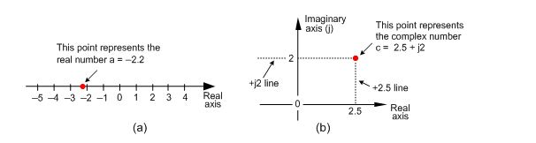
Figure 1. An graphical interpretation of a real number and a complex number.
A complex number, c, is shown in Figure 1(b) where it's also represented as a point. However, complex numbers are not restricted to lie on a one-dimensional line, but can reside anywhere on a two-dimensional plane. That plane is called the complex plane (some mathematicians like to call it an Argand diagram), and it enables us to represent complex numbers having both real and imaginary parts. For example in Figure 1(b), the complex number c = 2.5 + j2 is a point lying on the complex plane on neither the real nor the imaginary axis. We locate point c by going +2.5 units along the real axis and up +2 units along the imaginary axis. Think of those real and imaginary axes exactly as you think of the East-West and North-South directions on a road map.
We'll use a geometric viewpoint to help us understand some of the arithmetic of complex numbers. Taking a look at Figure 2, we can use the trigonometry of right triangles to define several different ways of representing the complex number c.
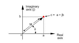
Figure 2 The phasor representation of complex number c = a + jb on the complex plane.
Our complex number c is represented in a number of different ways in the literature, such as:
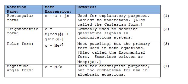
Eqs. (3) and (4) remind us that c can also be considered the tip of a phasor on the complex plane, with magnitude M, oriented in the direction of φ radians relative to the positive real axis as shown in Figure 2. Keep in mind that c is a complex number and the variables a, b, M, and φ are all real numbers. The magnitude of c, sometimes called the modulus of c, is

[Trivia question: In what 1939 movie, considered by many to be the greatest movie ever made, did a main character attempt to quote Eq. (5)?]

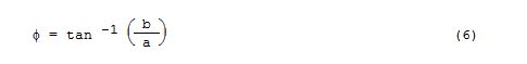
OK, back to business. The phase angle φ, or argument, is the arctangent of the ratio ![]() , or
, or
If we set Eq. (3) equal to Eq. (2), Mejφ = M[cos(φ) + jsin(φ)] , we can state what's named in his honor and now called one of Euler's identities as:

The suspicious reader should now be asking, "Why is it valid to represent a complex number using that strange expression of the base of the natural logarithms, e, raised to an imaginary power?" We can validate Eq. (7) as did the world's greatest expert on infinite series, Herr Leonard Euler, by plugging jφ in for z in the series expansion definition of ez in the top line of Figure 3. That substitution is shown on the second line. Next we evaluate the higher orders of j to arrive at the series in the third line in the figure. Those of you with elevated math skills like Euler (or those who check some math reference book) will recognize that the alternating terms in the third line are the series expansion definitions of the cosine and sine functions.
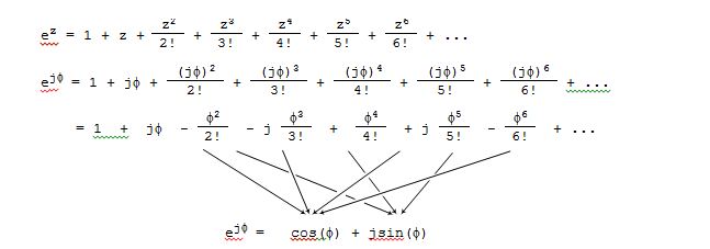
Figure 3 One derivation of Euler's equation using series expansions for ez, cos(φ), and sin(φ).
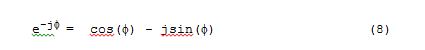
Figure 3 verifies Eq. (7) and our representation of a complex number using the Eq. (3) polar form: Mejφ. If you substitute -jφ for z in the top line of Figure 3, you'd end up with a slightly different, and very useful, form of Euler's identity:
The polar form of Eqs. (7) and (8) benefits us because:
- It simplifies mathematical derivations and analysis,
-- turning trigonometric equations into the simple algebra of exponents,
-- math operations on complex numbers follow exactly the same rules as real numbers.
- It makes adding signals merely the addition of complex numbers (vector addition),
- It's the most concise notation,
- It's indicative of how digital communications system are implemented, and described in the literature.
We'll be using Eqs. (7) and (8) to see why and how quadrature signals are used in digital communications applications. But first, let’s take a deep breath and enter the Twilight Zone of that 'j' operator.
You've seen the definition j = √-1 before. Stated in words, we say that j represents a number when multiplied by itself results in a negative one. Well, this definition causes difficulty for the beginner because we all know that any number multiplied by itself always results in a positive number.
Unfortunately DSP textbooks often define the symbol j and
then, with justified haste, swiftly carry on with all the ways
that the j operator can be used to analyze sinusoidal signals.
Readers soon forget about the question: What does j = √-1
actually mean?
Well, √-1 had been on the mathematical scene for some time, but wasn't taken seriously until it had to be used to solve cubic equations in the sixteenth century. [1], [2] Mathematicians reluctantly began to accept the abstract concept of 1, without having to visualize it, because its mathematical properties were consistent with the arithmetic of normal real numbers.
It was Euler's equating complex numbers to real sines and cosines, and Gauss' brilliant introduction of the complex plane, that finally legitimized the notion of √-1 to Europe's mathematicians in the eighteenth century. Euler, going beyond the province of real numbers, showed that complex numbers had a clean consistent relationship to the well-known real trigonometric functions of sines and cosines. As Einstein showed the equivalence of mass and energy, Euler showed the equivalence of real sines and cosines to complex numbers. Just as modern-day physicists don’t know what an electron is but they understand its properties, we’ll not worry about what 'j' is and be satisfied with understanding its behavior. For our purposes, the j operator means rotate a complex number by 90o counterclockwise. (For you good folk in the UK, counterclockwise means anti-clockwise.) Let's see why.
We'll get comfortable with the complex plane representation of imaginary numbers by examining the mathematical properties of the j = √-1 operator as shown in Figure 4.
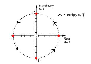
Figure 4. What happens to the real number 8 when you start multiplying it by j.
Multiplying any number on the real axis by j results in an imaginary product that lies on the imaginary axis. The example in Figure 4 shows that if +8 is represented by the dot lying on the positive real axis, multiplying +8 by j results in an imaginary number, +j8, whose position has been rotated 90o counterclockwise (from +8) putting it on the positive imaginary axis. Similarly, multiplying +j8 by j results in another 90o rotation yielding the -8 lying on the negative real axis because j2 = -1. Multiplying -8 by j results in a further 90o rotation giving the -j8 lying on the negative imaginary axis. Whenever any number represented by a dot is multiplied by j, the result is a counterclockwise rotation of 90o. (Conversely, multiplication by -j results in a clockwise rotation of -90o on the complex plane.)
If we let φ = π/2 in Eq. 7, we can say that
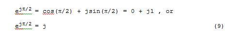
Here's the point to remember. If you have a single complex number, represented by a point on the complex plane, multiplying that number by j or by ejπ/2 will result in a new complex number that's rotated 90o counterclockwise (CCW) on the complex plane. Don't forget this, as it will be useful as you begin reading the literature of quadrature processing systems!
Let's pause for a moment here to catch our breath. Don't worry if the ideas of imaginary numbers and the complex plane seem a little mysterious. It's that way for everyone at first—you'll get comfortable with them the more you use them. (Remember, the j-operator puzzled Europe's heavyweight mathematicians for hundreds of years.) Granted, not only is the mathematics of complex numbers a bit strange at first, but the terminology is almost bizarre. While the term imaginary is an unfortunate one to use, the term complex is downright weird. When first encountered, the phrase complex numbers makes us think 'complicated numbers'. This is regrettable because the concept of complex numbers is not really all that complicated. Just know that the purpose of the above mathematical rigmarole was to validate Eqs. (2), (3), (7), and (8). Now, let's (finally!) talk about time-domain signals.
Representing Real Signals Using Complex Phasors
OK, we now turn our attention to a complex number that is a function time. Consider a number whose magnitude is one, and whose phase angle increases with time. That complex number is the ej2πfot point shown in Figure 5(a). (Here the 2πfo term is frequency in radians/second, and it corresponds to a frequency of fo cycles/second where fo is measured in Hertz.) As time t gets larger, the complex number's phase angle increases and our number orbits the origin of the complex plane in a CCW direction. Figure 5(a) shows the number, represented by the black dot, frozen at some arbitrary instant in time. If, say, the frequency fo = 2 Hz, then the dot would rotate around the circle two times per second. We can also think of another complex number e-j2πfot (the white dot) orbiting in a clockwise direction because its phase angle gets more negative as time increases.
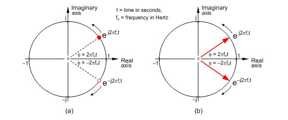
Figure 5. A snapshot, in time, of two complex numbers whose exponents change with time.
Let's now call our two ej2πfot and e-j2πfot complex expressions quadrature signals. They each have quadrature real and imaginary parts, and they are both functions of time. Those ej2πfot and e-j2πfot expressions are often called complex exponentials in the literature.
We can also think of those two quadrature signals, ej2πfot and e-j2πfot, as the tips of two phasors rotating in opposite directions as shown in Figure 5(b). We're going to stick with this phasor notation for now because it'll allow us to achieve our goal of representing real sinusoids in the context of the complex plane. Don't touch that dial!
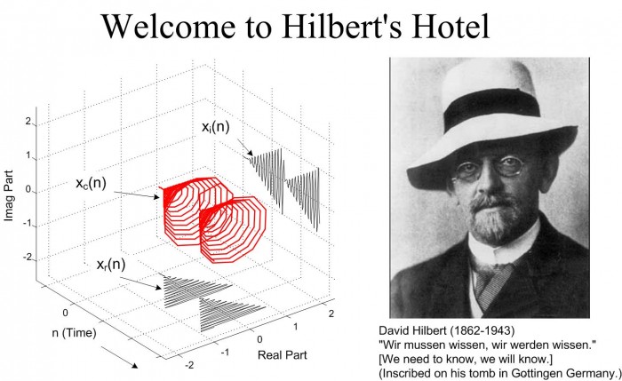
To ensure that we understand the behavior of those phasors, Figure 6(a) shows the three-dimensional path of the ej2πfot phasor as time passes. We've added the time axis, coming out of the page, to show the spiral path of the phasor. Figure 6(b) shows a continuous version of just the tip of the ej2πfot phasor. That ej2πfot complex number, or if you wish, the phasor's tip, follows a corkscrew path spiraling along, and centered about, the time axis. The real and imaginary parts of ej2πfot are shown as the sine and cosine projections in Figure 6(b).
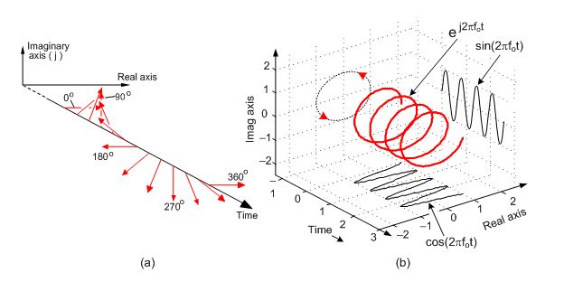
Figure 6. The motion of the ej2πfot phasor (a), and phasor 's tip (b).
Return to Figure 5(b) and ask yourself: "Self, what's the vector sum of those two phasors as they rotate in opposite directions?" Think about this for a moment... That's right, the phasors' real parts will always add constructively, and their imaginary parts will always cancel. This means that the summation of these ej2πfot and e-j2πfot phasors will always be a purely real number. Implementations of modern-day digital communications systems are based on this property!
To emphasize the importance of the real sum of these two complex sinusoids we'll draw yet another picture. Consider the waveform in the three-dimensional Figure 7 generated by the sum of two half-magnitude complex phasors, ej2πfot/2 and e-j2πfot/2, rotating in opposite directions around, and moving down along, the time axis.
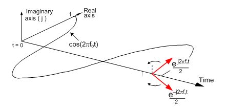
Figure 7. A cosine represented by the sum of two rotating complex phasors.
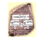
Thinking about these phasors, it's clear now why the cosine wave can be equated to the sum of two complex exponentials by
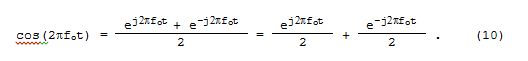
Eq. (10), a well-known and important expression, is also called one of Euler's identities. We could have derived this identity by solving Eqs. (7) and (8) for jsin(φ), equating those two expressions, and solving that final equation for cos(φ). Similarly, we could go through that same algebra exercise and show that a real sine wave is also the sum of two complex exponentials as
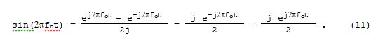
Look at Eqs. (10) and (11) carefully. They are the standard expressions for a cosine wave and a sine wave, using complex notation, seen throughout the literature of quadrature communications systems. To keep the reader's mind from spinning like those complex phasors, please realize that the sole purpose of Figures 5 through 7 is to validate the complex expressions of the cosine and sine wave given in Eqs. (10) and (11). Those two equations, along with Eqs. (7) and (8), are the Rosetta Stone of quadrature signal processing.
We can now easily translate, back and forth, between real sinusoids and complex exponentials. Again, we are learning how real signals, that can be transmitted down a coax cable or digitized and stored in a computer's memory, can be represented in complex number notation. Yes, the constituent parts of a complex number are each real, but we're treating those parts in a special way - we're treating them in quadrature.
Representing Quadrature Signals In the Frequency Domain
Now that we know something about the time-domain nature of quadrature signals, we're ready to look at their frequency-domain descriptions. This material is critical because we’ll add a third dimension, time, to our normal two-dimensional frequency domain plots. That way none of the phase relationships of our quadrature signals will be hidden from view. Figure 8 tells us the rules for representing complex exponentials in the frequency domain.
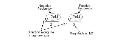
Figure 8. Interpretation of complex exponentials.
We'll represent a single complex exponential as a narrowband impulse located at the frequency specified in the exponent. In addition, we'll show the phase relationships between the spectra of those complex exponentials along the real and imaginary axes of our complex frequency domain representation. With all that said, take a look at Figure 9.
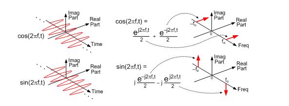
Figure 9. Complex frequency domain representation of a cosine wave and sine wave.
See how a real cosine wave and a real sine wave are depicted in our complex frequency domain representation on the right side of Figure 9. Those bold arrows on the right of Figure 9 are not rotating phasors, but instead are frequency-domain impulse symbols indicating a single spectral line for a single complex exponential ej2πfot. The directions in which the spectral impulses are pointing merely indicate the relative phases of the spectral components. The amplitude of those spectral impulses are 1/2. OK ... why are we bothering with this 3-D frequency-domain representation? Because it's the tool we'll use to understand the generation (modulation) and detection (demodulation) of quadrature signals in digital (and some analog) communications systems, and those are two of the goals of this tutorial. However, before we consider those processes let's validate this frequency-domain representation with a little example.
Figure 10 is a straightforward example of how we use the complex frequency domain. There we begin with a real sine wave, apply the j operator to it, and then add the result to a real cosine wave of the same frequency. The final result is the single complex exponential ej2πfot illustrating graphically Euler's identity that we stated mathematically in Eq. (7).
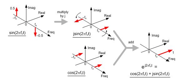
Figure 10. Complex frequency-domain view of Euler's: ej2πfot = cos(2πfot) + jsin(2πfot).
On the frequency axis, the notion of negative frequency is seen as those spectral impulses located at -2πfo radians/sec on the frequency axis. This figure shows the big payoff: When we use complex notation, generic complex exponentials like ej2πft and e-j2πft are the fundamental constituents of the real sinusoids sin(2πft) or cos(2πft). That's because both sin(2πft) and cos(2πft) are made up of ej2πft and e-j2πft components. If you were to take the discrete Fourier transform (DFT) of discrete time-domain samples of a sin(2πfot) sine wave, a cos(2πfot) cosine wave, or a ej2πfot complex sinusoid and plot the complex results, you'd obtain exactly those narrowband impulses in Figure 10.
If you understand the notation and operations in Figure 10, pat yourself on the back because you know a great deal about the nature and mathematics of quadrature signals.
Bandpass Quadrature Signals In the Frequency Domain
In quadrature processing, by convention, the real part of the spectrum is called the in-phase component and the imaginary part of the spectrum is called the quadrature component. The signals whose complex spectra are in Figure 11(a), (b), and (c) are real, and in the time domain they can be represented by amplitude values that have nonzero real parts and zero-valued imaginary parts. We're not forced to use complex notation to represent them in the time domain—the signals are real.
Real signals always have positive and negative frequency spectral components. For any real signal, the positive and negative frequency components of its in-phase (real) spectrum always have even symmetry around the zero-frequency point. That is, the in-phase part's positive and negative frequency components are mirror images of each other.
Conversely, the positive and negative frequency components of its quadrature (imaginary) spectrum are always negatives of each other. This means that the phase angle of any given positive quadrature frequency component is the negative of the phase angle of the corresponding quadrature negative frequency component as shown by the thin solid arrows in Figure 11(a). This 'conjugate symmetry' is the invariant nature of real signals when their spectra are represented using complex notation.
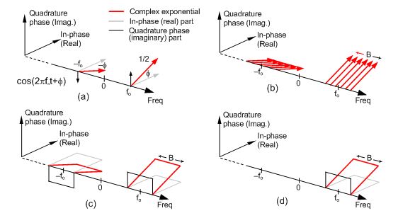
Figure 11. Quadrature representation of signals: (a) Real sinusoid cos(2πfot + φ), (b) Real bandpass signal containing six sinusoids over bandwidth B; (c) Real bandpass signal containing an infinite number of sinusoids over bandwidth B Hz; (d) Complex bandpass signal of bandwidth B Hz.
Let's remind ourselves again, those bold arrows in Figure 11(a) and (b) are not rotating phasors. They're frequency-domain impulse symbols indicating a single complex exponential ej2πft. The directions in which the impulses are pointing show the relative phases of the spectral components.
As for the positive-frequency only spectrum in Figure 11(d), this is the spectrum of a complex-valued analog time-domain bandpass signal. And that signal does not exhibit spectral symmetry centered around zero Hz, as do real-valued time-domain signals, because it has no negative-frequency spectral energy.
There's an important principle to keep in mind before we continue. Multiplying a time signal by the complex exponential ej2πfot, what we can call quadrature mixing (also called complex mixing), shifts that signal's spectrum upward in frequency by fo Hz as shown in Figure 12 (a) and (b). Likewise, multiplying a time signal by e-j2πfot shifts that signal's spectrum down in frequency by fo Hz.
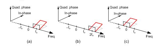
Figure 12. Quadrature mixing of a signal: (a) Spectrum of a complex signal x(t), (b) Spectrum of x(t)ej2πfot, (c) Spectrum of x(t)e-j2πfot.
We'll use that principle to understand the following example.
A Quadrature-Sampling Example
We can use all that we've learned so far about quadrature signals by exploring the process of quadrature-sampling. Quadrature-sampling is the process of digitizing a continuous (analog) bandpass signal and translating its spectrum to be centered at zero Hz. Let's see how this popular process works by thinking of a continuous bandpass signal, of bandwidth B, centered about a carrier frequency of fc Hz.
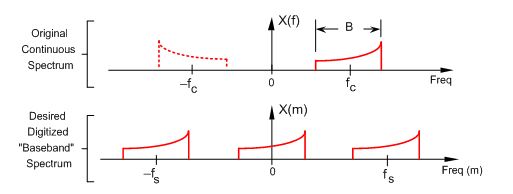
Figure 13. The 'before and after' spectra of a quadrature-sampled signal.
Our goal in quadrature-sampling is to obtain a digitized version of the analog bandpass signal, but we want that digitized signal's discrete spectrum centered about zero Hz, not fc Hz. That is, we want to mix a time signal with e-j2πfct to perform complex down-conversion. The frequency fs is the digitizer's sampling rate in samples/second. We show replicated spectra at the bottom of Figure 13 just to remind ourselves of this effect when A/D conversion takes place.
OK, ... take a look at the following quadrature-sampling block diagram known as I/Q demodulation (or 'Weaver demodulation' for those folk with experience in communications theory) shown at the top of Figure 14. That arrangement of two sinusoidal oscillators, with their relative 90o phase difference, is often called a quadrature-oscillator.
Those ej2πfct and e-j2πfct terms in that busy Figure 14 remind us that the constituent complex exponentials comprising a real cosine duplicates each part of the Xbp(f) spectrum to produce the Xi(f) spectrum. The Figure shows how we get the filtered continuous in-phase portion of our desired complex quadrature signal. By definition, those Xi(f) and I(f) spectra are treated as 'real only'.
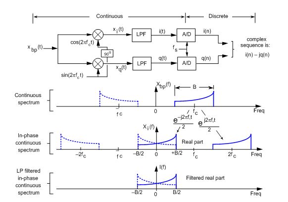
Figure 14. Quadrature-sampling block diagram and spectra within the in-phase (upper) signal path.
Likewise, Figure 15 shows how we get the filtered continuous quadrature phase portion of our complex quadrature signal by mixing xbp(t) with sin(2πfct).
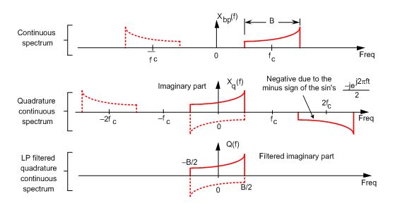
Figure 15. Spectra within the quadrature phase (lower) signal path of the block diagram.
Here's where we're going: I(f)–jQ(f) is the spectrum of a complex replica of our original bandpass signal xbp(t). We show the addition of those two spectra in Figure 16.
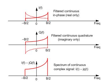
Figure 16. Combining the I(f) and Q(f) spectra to obtain the desired 'I(f)–jQ(f)' spectra.
This typical depiction of quadrature-sampling seems like mumbo jumbo until you look at this situation from a three-dimensional standpoint, as in Figure 17, where the –j factor rotates the 'imaginary-only' Q(f) by –90o, making it 'real-only'. This –jQ(f) is then added to I(f).
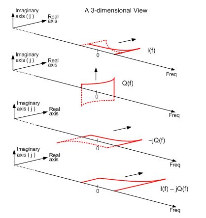
Figure 17. 3-D view of combining the I(f) and Q(f) spectra to obtain the I(f)–jQ(f) spectra.
The complex spectrum at the bottom Figure 18 shows what we wanted, a digitized version of the complex bandpass signal centered about zero Hz.
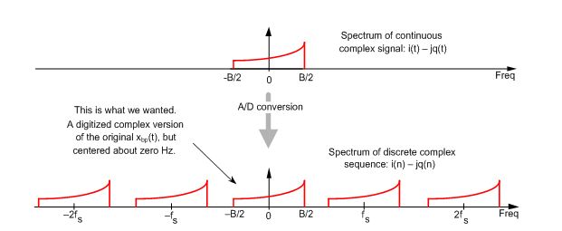
Figure 18. The continuous complex signal i(t)–q(t) is digitized to obtain the discrete i(n)–jq(n).
Some advantages of this quadrature-sampling scheme are:
• Each A/D converter operates at half the sampling rate of standard real-signal sampling,
• In many hardware implementations operating at lower clock rates save power.
• For a given fs sampling rate, we can capture wider-band analog signals.
• Quadrature sequences make FFT processing more efficient due to covering a wider frequency range than when an FFT’s input is a real-valued sequence.
• Because quadrature sequences are effectively oversampled by a factor of two, signal squaring operations are possible without the need for upsampling.
• Knowing the phase of signals enables coherent processing.
• Quadrature sampling makes it much easier to very accurately measure the instantaneous magnitude (AM demodulation), instantaneous phase (phase demodulation), and instantaneous frequency (FM demodulation) of the xbp(t) input signal in Figure 14.
Returning to the Figure 14 block diagram reminds us of an important characteristic of quadrature signals. We can send an analog quadrature signal to a remote location. To do so we use two coax cables on which the two real i(t) and q(t) signals travel. (To transmit a discrete time-domain quadrature sequence, we'd need two multi-conductor ribbon cables as indicated by Figure 19.)
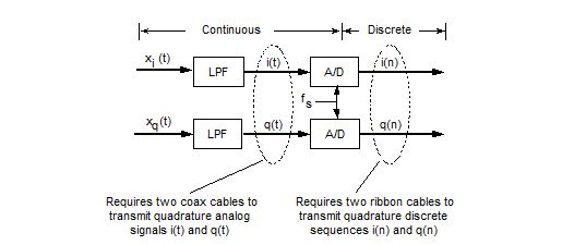
Figure 19. Reiteration of how quadrature signals comprise two real parts.
To appreciate the physical meaning of our discussion here, let's remember that a continuous quadrature signal xc(t) = i(t) + jq(t) is not just a mathematical abstraction. We can generate xc(t) in our laboratory and transmit it to the lab down the hall. All we need is two sinusoidal signal generators, set to the same frequency fo. (However, somehow we have to synchronize those two hardware generators so that their relative phase shift is fixed at 90o.) Next we connect coax cables to the generators' output connectors and run those two cables, labeled 'i(t)' for our cosine signal and 'q(t)' for our sine wave signal, down the hall to their destination.
Now for a two-question pop quiz. In the other lab, what would we see on the screen of an oscilloscope if the continuous i(t) and q(t) signals were connected to the horizontal and vertical input channels, respectively, of the scope? (Remembering, of course, to set the scope's Horizontal Sweep control to the 'External' position.)
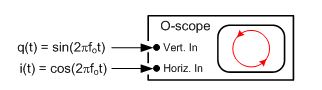
Figure 20. Displaying a quadrature signal using an oscilloscope.
Next, what would be seen on the scope's display if the cables were mislabeled and the two signals were inadvertently swapped?
The answer to the first question is that we’d see a bright 'spot' rotating counterclockwise in a circle on the scope's display. If the cables were swapped, we'd see another circle, but this time it would be orbiting in a clockwise direction. This would be a neat little demonstration if we set the signal generators' fo frequencies to, say, 1 Hz.
This oscilloscope example helps us answer the important question, "When we work with quadrature signals, how is the j-operator implemented in hardware?” The answer is we can’t go to Radio Shack and buy a j-operator and solder it to a circuit board. The j-operator is implemented by how we treat the two signals relative to each other. We have to treat them orthogonally such that the in-phase i(t) signal represents an East-West value, and the quadrature phase q(t) signal represents an orthogonal North-South value. (By orthogonal, I mean that the North-South direction is oriented exactly 90o relative to the East-West direction.) So in our oscilloscope example the j-operator is implemented merely by how the connections are made to the scope. The in-phase i(t) signal controls horizontal deflection and the quadrature phase q(t) signal controls vertical deflection. The result is a two-dimensional quadrature signal represented by the instantaneous position of the dot on the scope's display.
A person in the lab down the hall who's receiving, say, the discrete sequences i(n) and q(n) has the ability to control the orientation of the final complex spectra by adding or subtracting the jq(n) sequence as shown in Figure 21.
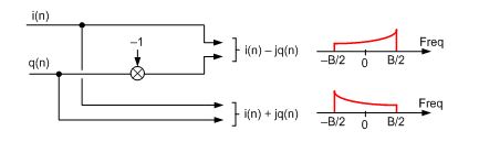
Figure 21. Using the sign of q(n) to control spectral orientation.
The top path in Figure 21 is equivalent to multiplying the original xbp(t) by e-j2πfct, and the bottom path is equivalent to multiplying the xbp(t) by ej2πfct. Therefore, had the quadrature portion of our quadrature-oscillator at the top of Figure 14 been negative, sin(2πfct), the resultant complex spectra would be flipped (about 0 Hz) from those spectra shown in Figure 21.
While we’re thinking about flipping complex spectra, let’s remind ourselves that there are two simple ways to reverse (invert) an x(n) = i(n) + jq(n) sequence’s spectral magnitude. As shown in Figure 21, we can perform conjugation to obtain an x'(n) = i(n) jq(n) with an inverted magnitude spectrum. The second method is to swap x(n)’s individual i(n) and q(n) sample values to create a new sequence y(n) = q(n) + ji(n) whose spectral magnitude is inverted from x(n)’s spectral magnitude. (Note, while x'(n)’s and y(n)’s spectral magnitudes are equal, their spectral phases are not equal.)
Conclusions
This ends our little quadrature signals tutorial. We learned that using the complex plane to visualize the mathematical descriptions of complex numbers enabled us to see how quadrature and real signals are related. We saw how three-dimensional frequency-domain depictions help us understand how quadrature signals are generated, translated in frequency, combined, and separated. Finally we reviewed an example of quadrature-sampling and two schemes for inverting the spectrum of a quadrature sequence.

References
[1] D. Struik, A Concise History of Mathematics, Dover Publications, NY, 1967.
[2] D. Bergamini, Mathematics, Life Science Library, Time Inc., New York, 1963.
[3] N. Boutin, "Complex Signals," RF Design, December 1989.
Answer to trivia question just following Eq. (5) is: The scarecrow in The Wizard of Oz.
Have you heard this little story?
While in Berlin, Leonhard Euler was often involved in philosophical debates, especially with Voltaire. Unfortunately, Euler's philosophical ability was limited and he often blundered to the amusement of all involved. However, when he returned to Russia, he got his revenge. Catherine the Great had invited to her court the famous French philosopher Diderot, who to the chagrin of the czarina, attempted to convert her subjects to atheism. She asked Euler to quiet him. One day in the court, the French philosopher, who had no mathematical knowledge, was informed that someone had a mathematical proof of the existence of God. He asked to hear it. Euler then stepped forward and stated: "Sir, ![]() , hence God exists; reply!" Diderot had no idea what Euler was talking about. However, he did understand the chorus of laughter that followed and soon after returned to France.
, hence God exists; reply!" Diderot had no idea what Euler was talking about. However, he did understand the chorus of laughter that followed and soon after returned to France.
Although it's a cute story, serious math historians don't believe it. They know that Diderot did have some mathematical knowledge and they just can’t imagine Euler clowning around in that way.


- Comments
- Write a Comment Select to add a comment

You silver-tongued devil. Hope all is well with you.
[-Rick-]
From Figure 14, does the signal after ADC "i(n) - jq(n)" is implemented simply by subtracting digital samples i(n) from q(n)?
I'm wondering what are the consequences if I do not "i(n) - jq(n)", while having the positive and negative frequency spectrum overlapping after down-converted to DC in Figure 14. Does this corrupt the signal if the "negative i" signal is not filtered off/ subtracted from the inverted image in q?
Through my MATLAB simulation of downconverting the GFSK modulated signal to DC using I/Q, even if the (+i) and (-i) signal overlapped at DC, I can still recover the phase of the signal perfectly by arctan(q/i). Does this mean the overlapping of negative and positive frequency spectrum at DC does not corrupt the actual signal?
My assumption is that the upper side and lower side of the modulated bandpass filter do not happen at the same time. For example when "1" is transmitted, the upper sideband of positive frequency exist from 0 to BW/2 while the inverted frequency spectrum of negative frequency exist from -BW/2 to 0, hence there's no overlapping in fact?
Thanks for reading this :)
Dave Comer
The top of Figure 15 is the spectrum of the input analog bandpass signal. Negative-freq spectral energy is shown by a dashed curve.
The center of Figure 15 is the spectrum of the output of the bottom mixer in our Figure 14 block diagram. Notice at the bottom right of Figure 9 that a real-valued sine wave is equivalent to a positive-freq exponential and a negative-freq exponential. BUT, notice that the positive-freq exponential part of a real sine wave is 180 degrees out of phase relative to the negative-freq exponential part.
So when you multiply a real-valued bandpass signal by a sine wave, half the bandpass signal's spectral energy is translated up in frequency and half the bandpass signal's spectral energy is translated down in frequency.
To quote Ardeth Bay in the 1999 movie The Mummy, "Know this!" The up-translated spectral energy is 180 degrees out of phase relative to the down-translated spectral energy. That super-important characteristic is shown in the center of Figure 15 where spectral energy below the horizontal axis is 180 degrees out of phase with spectral energy above the horizontal axis.
I presume you understand the bottom part of Figure 15. I hope what I've written makes sense. If not, let me know, OK?
Amazing article! Never thought complicated mathematics can be explained in such a concise way as well as thorough explanation from concept to implementation.
Thank you so much!
If I may, I want to ask you a question about representing complex signal as real signals.
For example in QAM modulation, you have complex data, say, Z(t)=I(t)+jQ(t). To transmit this complex we modulate it and take the real component.
I.e.: we transmit the signal R(t) = Real{Z(t).e^(jft)}. Where 'f' is the carrier frequency. Then in the receiver side we mix this signal with sine and cosing, HPF it and extract I(t) and Q(t). This is fine.
Now, is there a way to do this in baseband? Can we send the baseband signal Z(t) without modulating it? That is f=0. Because when f=0, only real part of Z(t) is sent and no information about Q(t) is sent. So there is no way we can reconstruct Q(t) at receiver side.
For example in ADSL, when we perform DFT, we mirror our N complex data points and conjugate them before doing the DFT. This results in a real 2N signal, which is baseband, and can be transmitted without any carrier modulation.
But if we have complex a complex baseband signal, am I correct to think that there is no way to represent this complex signal as a real signal? Is there any way we can transmit this signal without sending I(t) and Q(t) separately in two wires as in your example?
Thank you very much for great contributions.
Thanks
Thanks
Dear Mr. Lyons, this is a very good article. I have learned a lot from it, and it wasn't that much difficult.
However, it seems to me that your Figure 6 is not correct: comparing with the symbols shown in the previous figure (Figure 5), it should be a positive frequency, thus it should be a counter-clockwise spinning helix (or corkscrew), but it is a clockwise helix. It doesn't matter if we go along the increasing or decreasing direction of the time axis, because the helix would be the same, anyway, but the projection (the circle in perspective) at the bottom plane looks inverted when we look at it from the wrong side.
Well, I hope you can find some use for this comment. I sincerely enjoyed very much reading your fine article.
Mauricio
Retired professor of Chemistry
Hello mgconsta. Thank you for your kind words.
The spiral in my Figure 6(b) is rotating in the counter-clockwise direction. Notice that the spiral is coming up out of the page as time passes. That is, the positive-time axis is pointing upward at the reader.
Richard,
Excellent article. I'm confused about one thing. The bottom plot of figure 17 shows the entire spectra drawn on the real axis and nothing in the imaginary axis, however, the spectra is clearly complex. Does this mean that the complex spectra cannot be represented by a spectral decomposition of real and imaginary axes?
Thanks,
Frank
Hello Frank. Your question is very sensible. In my hypothetical example (Fig. 17) the spectrum at the bottom of Fig. 17 is indeed real-only, but the time samples (the inverse DFT of that real-only spectrum) are complex-valued because that spectrum is NOT symmetrical with respect to zero Hz.
Try this out in your software: create real-only symmetrical frequency-domain samples as f1 = [1 1 1 0 0 0 0 0 1 1]. The IDFT of the symmetrical real-only 'f1' spec samples will be a real-only time-domain sequence. Next create real-only asymmetrical freq samples as f2 = [1 1 1 0 0 0 0 0 1 1 1]. The IDFT of the asymmetrical real-only 'f2' spec samples will be a complex-valued time-domain sequence. I hope what I've written makes some sense.
Richard,
Thanks for that explanation. I might have a follow-on question about this.
Frank
Getting below in matlab. How do you define symmetrical samples? Is x below asymetrical?
>> x= [1,1,0,0]
x =
1 1 0 0
>> y=ifft(x);
>> y
y =
0.50000 + 0.00000i 0.25000 + 0.25000i 0.00000 + 0.00000i 0.25000 - 0.25000i
Excellent article Rick!
These explanations enhanced my understanding on this subject a lot.
The only term that puzzles me is the frequently used "frequency impulse". I understand the meaning, but humbly suggest the term "frequency component"instead. Impulse is more time-domain oriented in my opinion, and could be confused with "impulse response". No big thing, but could enhance the readability.
Thanks again for an amazing piece !
BR,
Bjørn
Hello Bjørn, thank you for your kind words.
You comment and suggestion are certainly sensible. Please allow me to contemplate your suggestion. (Words are "tricky", are they not?)
The figure 11d seems to suggest complex bandpass signal does not have any energy at negative frequency. Is it true?
Hello tusharpatel342. Yes, you are correct. The complex bandpass signal whose spectrum is shown in Figure 11(d) has no negative-frequency spectral energy.
The time-domain samples of that ideal bandpass signal are complex-valued, and if you performed an N-point DFT on N of those complex-valued time samples the spectral results would show no negative-frequency energy. (In the literature of DSP, such a signal is often called an "analytic signal.")
Thanks for quick relpy, Rick. Do all complex signals have this property?
A complex signal is one whose time-domains samples are complex valued. And such signals have spectra where the positive- and negative-frequency components do NOT have the conjugate symmetry of real-valued signals (real-values signals such as those conjugate-symmetric spectra shown in Figures 11(a), 11(b) & 11(c)).
Discrete complex signals can have negative-frequency energy such as the discrete signal whose spectrum is shown at the bottom of my Figure 18. (Notice the asymmetrical spectral magnitude of that discrete signal.) However, that particular complex signal is NOT an "analytic signal" because it has nonzero negative-frequency spectral energy.
So the answer to your question is, "No."
[By the way, years ago I read a scholarly mathematical paper describing the origin of the mathematical word "analytic", but I've since forgotten whatever it was that I read.]
Thanks Rick! BTW small anecdote, I took some DSP classes during my graduate studies at SJSU. My professor suggested your book (Understanding Digital Signal processing) for coursework. Since that day I became a big fan of yours. You do make DSP fun!!!
Hi tusharpatel342. Thanks for your kind words, I appreciate them.
San Jose State University, huh? Good for you. Are you still in the Bay area? I lived in Sunnyvale for many years (back then the traffic wasn't so bad). I live up in Auburn CA now.
By the way, if you own a copy of my "Understanding DSP" book, have a look at:
Hi Rick, yeah I arrived in San Jose in 2007 for my master study. I currently work in Sunnyvale. My company called Litepoint and we make testers for phy layer testing for different wireless technologies (WiFi/2g/3g/LTE/Bluetooth/NFC/WiGig/5G).And yes traffic has gone brutal lately. I've never been to Auburn CA, but believe traffic should be better than bay area.
Hi. Litepoint's location is just a few miles from where I lived. Looking at their web site, Litepoint's products look rather complicated to me. Good for you for working there. Who knows, maybe some day you and I will meet up one afternoon and splash some beer around.
I am beer fanatic and would love to meetup. Ping me if you come to Sunnyvale in future.
Rick,
I have this confusion for very long time. Most of communication system uses complex IQ modulation and complex IQ sampling. So if my signal BW is 2Ghz, receiver can use I and Q A/D sampling simultaneously each A/D running at 2.4Ghz to analyze 2Ghz bandwidth without compromising nqyist theorem. For some reason I can't understand this. I am so stuck to sampling rate should be >= 2*signal BW.
Can you help me understand this?
tusharpatel, the traditional Nyquist criterion, for digitizing real valued analog signals of positive-frequency bandwidth B Hz, says that the fs sample rate must be fs ≥ 2B Hz. So if B = 100 Hz, then a single A/D converter sampling process must generate no less than 200 output samples/second to satisfy Nyquist.
In this B = 100 Hz scenario, using the two-A/D converter sampling scheme in my Figure 14 would also generate no less than 200 output samples/second. That's because each A/D converter, sampling at fs = 100 Hz, is generating 100 samples/second. I hope that answers you question. If not, please let me know.
Hello Mr Lyons.
I want to know if this analytic signal (which is a complex-valued function of time), say x(t), has any relationship with the real signal that were sampled s(t) (which is a real-valued function). I just want to confirm if the analytic signal is obtained from the real one by means of the Hilbert Transform of s(t), H(s(t)), and if this analytic signal is
x(t) = s(t) + j H(s(t))
If that's true, does it mean that the in-phase part is the signal itself and the quadrature is its Hilbert Transform?
Assuming that the equation for x is right and thinking about the advantages that you list, does it mean that the only way of getting the phase information of s(t) is trough IQ processing? I'm a little bit confused about this and the equation before.
For example, if I'm using a mixer to process an RF signal without IQ processing, is the signal that I get s(t)? This wave can't give me the phase due to the lack of temporal reference, so I just represent the signal as a sum of two waveforms with the same frequency but shifted 90°: The in-phase and quadrature (the 90° shifting explains to me the 'j' in the equation above), but, if that's true, then the signal is actually x(t), no s(t)? The true amplitude of the signal received is that of s or that of x?
Thanks a lot for your time :)
Hi daandres. You wrote: "I just want to confirm if the analytic signal is obtained from the real one by means of the Hilbert Transform of s(t), H(s(t)), and if this analytic signal is
x(t) = s(t) + j H(s(t))
If that's true, does it mean that the in-phase part is the signal itself and the quadrature is its Hilbert Transform?"
daandres , I can confirm that what you wrote is correct. Your above equation was for a continuous (analog) signal. The discrete signal version of your equation is:
x(n) = s(n) + j H(s(n)).
You wrote: "does it mean that the only way of getting the phase information of s(t) is through IQ processing?"
There may be other ways to compute the instantaneous phase of a real-valued sinusoid, but off the top of my head I can't think of any way to estimate the instantaneous phase of your real s(n) sequence other than computing the instantaneous phase of your complex x(n) sequence.
Also, the whole notion of estimating the instantaneous phase of a real-valued signal only applies to real-valued signals containing just one sinusoid having a given frequency. If your real-valued input signal is the sum of two (or more) sinusoids, say a 1000 Hz sine wave plus a 1031.7763 Hz sine wave, then the notion of instantaneous phase makes no sense (has no meaning).
You wrote: " For example, if I'm using a mixer to process an RF signal without IQ processing, is the signal that I get s(t)?" The answer is "Yes." And that is assuming your RF signal is a single sinusoidal signal (a single sine wave).
You wrote: " This wave can't give me the phase due to the lack of temporal reference, so I just represent the signal as a sum of two waveforms with the same frequency but shifted 90°: The in-phase and quadrature (the 90° shifting explains to me the 'j' in the equation above)"
I'm uncomfortable with your use of the term "sum." The s(n) and H(s(n)) sequences are both real-valued. The x(n) sequence is a two-dimensional sequence where we agree that s(n) represents the East/West value of the two-dimensional x(n) signal and H(s(n)) represents the North/South value of the two-dimensional x(n) signal. At no time do we actually "sum" (add) the two real-valued s(n) and H(s(n)) sequences.
As for the " the lack of temporal reference", you are correct. In general, people typically estimate the instantaneous phase of an input real-valued sinusoid so they can compare that instantaneous phase to the instantaneous phase of some sort of "reference" sinusoid having the same frequency as the input sinusoid.
You wrote: "but, if that's true, then the signal is actually x(t), not s(t)? The true amplitude of the signal received is that of s or that of x?"
I'm not sure what your phrase "the signal" means. What do your words "the signal" mean? If you can ask your last question in a way that I can fully understand it then I'll do my best to answer it.
Hi Mr Lyons.
Thanks a lot for your quick an meaningful answer. I think that the relation between s and x is fully understood.
On the phase meaning, I would like to know: In the signal that you proposed, I can't say anything about the phase of the resulting signal, but still can talk about the phase of the single-frequency sinusoids that compose it (the phases of the 1000 Hz and 1031.7763 Hz sinusoids individually), right? (I think that this is the idea in coherent communications).
About the "sum" term that I used, this idea comes from what I saw in some YouTube videos (I leave you one of them at the end of my reply, the "sum" is explained at min 12:00, if you could look at it, it would be great). The main idea that they explain is you can take two sinusoids in quadrature and then sum both to get another sinusoid whose phase deppends on the relative amplitude of the original ones. The opposite is true and the wave (purple) can be decomposed in the in-phase part (yellow) and the quadrature part (green).
The same video could be useful to explain what I meaning with "the signal". When he summed the two in quadrature signals, he got another wave with more amplitude and intermediate phase, the purple one. This purple signal is what I'm meaning as "the signal". Am I misunderstanding something?
Thanks again for your time.
I think that video is more harmful than it is helpful. When he claims that the purple sine wave is the sum of the green and yellow sine waves, he is *NOT* correct. At the instant in time when the yellow wave has a value of zero the green and purple waves should have equal amplitudes. And that is not true in his video!! I'm surprised he didn't see that.
Also, I have *NEVER* seen an application of quadrature signal processing where we sum (add) the real and imaginary parts of a complex signal. So his entire explanation while viewing those green, yellow, and purple sine waves, while true, has *NOTHING* to do with quadrature processing. Because he now has you thinking about the nonsensical idea of adding the real and imaginary parts of a complex signal, I strongly suggest you ignore his *ENTIRE* explanation of those green, yellow, and purple sine waves and forget about the process of adding the real and imaginary parts of a complex signal.
When he showed Euler's equations I couldn't make any sense out of what he was saying regarding a local oscillator.
His discussion starting at time 18:03 in the video showing the following network:

may be correct, but I can't be sure without using software to model, and study, that network.
Hi again daandres.
One interesting and useful thing about your above video is the mention of the "Tayloe detector." I had never heard of such a quadrature detector before! There's a fair amount of info on the web discussing the Tayloe detector but one good web site is the following:
https://www.arrl.org/files/file/Technology/tis/inf...
Hi Mr Lyons,
I have been thinking a lot about your answer, and maybe it's me who mixed up the things in the wrong way.
I think that when he says quadrature, he is only saying that the two waves are 90° apart in phase. The same is done here (and he gives some applications)
About the non-matching amplitudes when the yellow is zero, look that the purple one is maximum when green and yellow cross (as expected because the slopes are equal in magnitude but opposite in sign), so this difference in amplitude might be a matter of scale (the grid on the background suggest that the purple is the double of the sum), and that scale difference might be explained if we consider that the mixer splits the amplitude of the sine wave in two halves, and the IF filer removes one of them:
For the in-phase (yellow):
sin(ws t) cos(wlo t) = 1/2 sin[(ws + wlo) t] + 1/2 sin[(ws - wlo) t]
For the quadrature (green):
sin(ws t) sin(wlo t) = 1/2 cos[(ws - wlo) t] - 1/2 cos[(ws + wlo) t]
where ws and wlo are the angular frequencies of the signal and local oscilator respectively. This of course assumes that the network whose diagram you posted in your previous reply is correct (and I'm thinking that this is the case, I saw the same diagram to represent the detector in radars -here for example- and in the article you shared with me).
On the other hand, I still have this question: In the signal that you proposed before (the one composed of 1000 Hz and 1031.77Hz), I
can't say anything about the phase of the resulting signal, but still
can talk about the phase of the single-frequency sinusoids that compose
it?
And with your previous reply another question arised, it's a little bit philosophical. As you say in your post at the beginning of the Band pass Quadrature Signals section, refering to real-valued signals: "We're not forced to use complex notation to represent them in the time domain"; so in the case of real-valued signals, is the quadrature component something real? Is it just a mathematical thing that we use to simplify the analysis and get all the information from the signal? Is it both?
Finally, I would like to give my deepest thanks for your help.
Hi daandres.
I think you are correct regarding the amplitude of the purple sine wave in your first video.
In one of my previous Comments I wrote:
"Also, the whole notion of estimating the instantaneous phase of a real-valued signal only applies to real-valued signals containing just one sinusoid having a given frequency. If your real-valued input signal is the sum of two (or more) sinusoids, say a 1000 Hz sine wave plus a 1031.7763 Hz sine wave, then the notion of instantaneous phase makes no sense (has no meaning)."
Thinking more about what I wrote I believe I should retract (take back) my above italicized words. I say that because I thought about frequency modulated (FM) signals. We can receive an FM signal, use the Hilbert transform to generate a complex-valued version of the FM signal, frequency translate the complex-valued version of the FM signal down to be centered at zero Hz creating a complex-valued baseband signal, and then compute the instantaneous phase of the complex-valued baseband signal. My point is, that complex-valued baseband signal contains multiple spectral components but it is still valid (still meaningful) to discuss the instantaneous phase of the complex-valued baseband signal. So that's why I want to retract my above italicized words.
Also, earlier this morning in a textbook I found an application where a modulated real-valued cosine wave of frequency Fo is added (summed) to a modulated real-valued sine wave of the same Fo frequency. That application is in the transmission of a Quadrature Amplitude Modulation (QAM) digital communication system. And then a few minutes ago I viewed your second video, and there it was—--a description of QAM!!
Regarding your question in the last paragraph of your comment: In my blog I wrote: "The signals whose complex spectra are in Figure 11(a), (b), and (c) are real, and in the time domain they can be represented by amplitude values that have nonzero real parts and zero-valued imaginary parts. We're not forced to use complex notation to represent them in the time domain—the signals are real." By that I meant: We can think of all signals as being complex-valued having a real part and an imaginary part. And we can think of a single complex signal sample as: x = A + jB
However, real-valued signals are complex-valued signals where the imaginary parts is always zero. So rather than referring to a single sample of a real-valued signal as: y = A + j0, we merely refer to that real-valued 'y' number as: y = A. That is, we can represent the real-valued sample 'y' in two ways:
y = A + j0[complex notation]
y = A[real-only notation]
For a real-valued signal sample people do NOT use the 'y = A + j0' complex notation', they use the 'y = A' real-only notation.
So from a philosophical standpoint I'd say: In complex notation a real-valued sample has an imaginary part and that imaginary part is always zero. In real-only notation a real-valued sample has no imaginary part. In real-only notation imaginary parts do not exist.
Hi Mr Lyons,
I really appreciate your answers, they have helped me a lot to organize and polish my ideas.
I think I understand what you're saying about the philosophical meaning of the quadrature component in the real-valued signal. So I would like to change my original question for this: Given that the analytical signal is the easy way to get the phase and amplitude of the real-valued signal, Is the analytical signal something real? Is it just a mathematical thing that we use to simplify the analysis and get all the information from the real-valued signal? Is it both?
"Given that the analytical signal is the easy way to get the phase and amplitude of the real-valued signal, Is the analytical signal something real? Is it just a mathematical thing that we use to simplify the analysis and get all the information from the real-valued signal? Is it both?"
Let me reword your question into what I think you are asking of me. My rewording of your question is:
"Given that the analytical signal is A way to ESTIMATE the INSTANTANEOUS phase and WHAT WE CALL THE "INSTANTANEOUS MAGNITUDE" of the real-valued signal, DOES AN ANALYTICAL SIGNAL ACTUALLY EXIST IN OUR PHYSICAL WORLD? OR IS THE ANALYTICAL SIGNAL JUST A MATHEMATICAL CONCEPT that we use to simplify the analysis and get all the information from the real-valued signal? Is it both?"
My answer is: It is both. We can, and do, represent an analytic (complex-valued) signal using mathematical equations. And an analytic signal definitely exists in our physical world. At time 12:10 in your first video the was a real-valued cosine wave transmitted through a coax cable and displayed on the oscilloscope as the green trace. That real-valued cosine wave voltage exists in our physical world. At the same time in the video there was another real-valued signal, a sine wave, transmitted through a *separate* coax cable and displayed on the oscilloscope as the yellow trace. That real-valued sine wave voltage also exists in our physical world. (Always remember, it takes two coax cables to transmit a single continuous analytic signal!)
The "analytic" (what we call "complex") idea comes from our agreement that we will create a 2-dimensional signal, ...a signal that has two parts exactly like a location on the Earth has two parts (latitude & longitude). And we agree that the cosine wave represents the fluctuating instantaneous East/West value of our 2-dimensional analytic signal. Likewise, we agree that the sine wave represents the fluctuating instantaneous North/South value of our 2-dimensional analytic signal.
In the video if the peak voltage of the cosine and sine wave voltages were 200 volts and you touched either coax cable's center conductor and shield at the same time you would be quickly and painfully aware that analytic signals exist in our physical world.
Hi Rick,
Once again excellent article. I have one question, I dont understand the sentence:
Each A/D converter operates at half the sampling rate of standard real-signal sampling
Do we somehow able to sample with frequency lower than the Nyquist, I mean the signal has still BW of B so the sampling rate is supposed to be 2B right?
Hello ctzof. Sorry for the possibly poor wording in my blog.
When we sample a real-valued analog signal of bandwidth B Hz, using a single A/D converter, the Fs sample rate must be no less than 2B Hz. But in my Figure 14 the two A/Ds each need only sample at an Fs rate of B Hz. So, ...those two A/Ds, which working together are sampling a complex-valued analog signal of bandwidth B Hz, are operating at half the traditional sampling rate as a single A/D sampling a real-valued analog signal of bandwidth B Hz.
I hope what I've written here makes sense to you.
Hi Rick,
Thanks for the response, I think it makes sense. Just for my understanding, to express things a little bit different. If we use a conventional mixer then the maximum frequency that we can use for this mixer is fc-B/2 to avoid mixing positive and negative part of the spectrum. This would make the BW of the signal double and it would inevitably require higher sampling rate. Is my way of thinking right?Darn. I'm not able to understand the scenario that you are describing. Can you post a block diagram of the processing you have in mind, or can you ask your question by referring to specific figures in my blog?
Hi Rick,
I've made a rough diagram for presenting my idea using conventional mixing. What I want mostly to understand is the benefits of quadrature conversion comparing to conventional. As you can see in the diagram by using a conventional mixer for for direct conversion down to base-band the two frequency spectrum overlap with each other and the original spectrum cannot be extracted anymore. To avoid this the maximum mixing frequency that we can use is fc-B/2 which in order to be sampled properly a sample rate of at least 2B has to be used. I hope this makes sense, please correct me if I am wrong.

Thanks
ctzof, I understand what you are saying. The top two panels of your figure are similar to the top two spectra in my Figure 14. Except in my figure I show both the down-conversion (downward freq translation) AND up-conversion (upward freq translation) that takes place during analog mixing of real-valued signals in the top path of the network at the top of my Figure 14. And yes, the spectral energy centered at zero Hz is "contaminated" in that top path. But the full (dual-path) quadrature sampling network at the top of Figure 14 enables us to eliminate that contamination and produce a uncontaminated spectrum centered at zero Hz as shown in Figures 16 & 17. That's the whole purpose of using quadrature sampling!
I list the advantages of quadrature sampling just below my Figure 18. The last bullet in that list should be emphasized. Quad sampling produces a complex-valued sequence (centered at zero Hz) that can be AM demodulated, FM demodulated, or phase demodulated VERY accurately in very straightforward (simple) ways. That's why quadratue sampling is popular in digital radios.
Regarding the bottom panel of your figure, yes, you can generate such a signal using a single analog mixer (followed by analog lowpass filtering) and a single A/D converter. But the disadvantages are that the A/D converter must sample at fs = 2B Hz, and the resulting real-valued discrete sequence is NOT easily, or particularly accurately, AM, FM, or PM demodulated.
Hi Rick,
That is clear enough,thank you for your time and once more (as in many othe DSP topics) meaningfull explanation.
Hi, Rick,
Very nice article to read!
Here I have 2 questions hope you could help:
1) It seems very critical for matching between I and Q channel, like gain and delay? How to specify the specifications on gain and delay matching?
2) We are working on touch sensor and what we apply is amplitude modulation. For demodulation, people would transfer the received signal to Digital by ADC first, then do I&Q demodulation. I tried to understand how resolution of ADC and processing clock of digital modulator impacts the overall performance, any thoughts?
Thank you again!
Athree
Hello Arthree. Sorry for my delayed reply--I just now read your post. I haven't studied the problems caused by I/Q gain and phase mismatch. I've never tried including attached files here in a "Reply" before, but below are a few PDF files that discuss I/Q mismatch. (Maybe they'll be useful to you Arthree.)
I-Q imbalance correction - Ellingson.pdf
Please forgive me but I do not understand your question. If you can re-ask your question and include more details of what you have in mind, I'll do my best to answer a new question.
My question is about correcting for “simulcast distortion” in radios (police, fire, etc.) caused by phase shifts in reception from antenna towers sending identical messages, but at varying distances from any mobile radio. Such radios have been standardized to a degree through an enormous set of standards published as APCO Project 25 by the Association of Public-Safety Communications Officials (many of whom represent the radio industry). It’s difficult to sort through the hodgepodge (maybe to protect the $5000 price of each Motorola mobile radio?) of standards (with some information proprietary), but my impression is that frequency-shift keying was the original standard, modified now to accommodate specific forms of QPSK and FSK for compatibility.
At least the original radio scanners (mainly in amateur use) were developed around FSK. The scanners often suffer excessively from simulcast distortion, whereas the expensive mobile transceivers in actual use evidently do not. In fact, there is now available a passive receiver (sold by Unication USA) that also seems completely free of this interference.
I understand that with QPSK there is a straightforward way of correcting for images from reflections that may be present in reception of signals from a single transmitter tower. My question is: Can simulcast distortion similarly be minimized, arising from phase-shifted versions of a signal?
I've written to APCO asking for any specifications stated regarding QPSK or FSK in Project 25. Will inform you if I get an answer.
Thanks,
David
Rick, Have you had any luck understanding my question, expanded in my Feb 15 message? Thanks, bartlesome
Hi bartlesome (David). I just now saw your Feb. 15th post.
I'm not a digital communications guy so I'm sorry to say that I cannot answer your question. I suggest you post your question on the "Forum" page of this dsprelated.com web site. There are subscribers to that "Forum" that are much more knowledgeable regarding "digital communications" than I. (For example, Eric Jacobsen, AKA Slartibartfast.)
You asked if I understood your Feb 15th question. Just so you know, here's my interpretation of your question:
"Some radio communications systems suffer from a kind of "phase shift" distortion where a receiver receives a desired signal plus (contaminated by) a phase-shifted version of the desired signal. This distortion can be caused in two ways: 1) when a receiver receives a signal directly from a single transmitting antenna plus a delayed signal reflected from a building; and 2) when two physically-separated antennas transmit the same signal (what could be called "simulcast distortion"). Rumor on the street has it that for QPSK-modulated signals the "reflected" type of phase shift distortion can be corrected. The question is: For QPSK-modulated signals is there a way to correct for the dual-transmitter simulcast distortion?"
Anyway David, the above is my interpretation of your question. I hope someone on the "Forum" can help you out.
[-Rick-]
Hi,
I have a fundamental question regarding Figure 13,14.
If I did have a complex bandpass signal at 2fo represented by x(t)exp(j*2pi*fo*t) (ie no negative spectrum) and I upconvert with exp(j*2*pi*fc*t) - again no negative spectrum, will the spectrum result only in positive frequency ?
If that's the case, why is there a negative spectrum(dotted spectrum) for Figure 13 ?
Suppose we did use the signal in Figure 12(d) we should be able to bring back the spectrum to x(t)exp(j*2pi*fo*t) by multiplying the spectrum with exp(-j*2*pi*fc*t) and then get x(t) by multiplying again with exp(-j*2pi*fo*t).
In Figure 14, xbp(f) is shown in positive and negative spectrum. What would the spectrum look like if the xbp(f) is a complex bandpass signal ? Is it possible to transmit x(t)exp(j*2pi*fo*t)*exp(j*2*pi*fc*t) with an antenna ?
Kindly explain.
[1] The top spectra in Figures 13 and 14 represent the spectrum of a hypothetical real-valued continuous (analog) bandpass signal. A signal that could be transmitted on a single coax cable. Because that signal is real-valued, and we're discussing quadrature signals, I chose to show that signal's positive- and negative-frequency spectral content. In Figure 14 I called that bandpass signal "x_bp(t)."
In the top spectra in Figures 13 and 14 I depicted the positive-frequency components with solid lines and negative-frequency components with dashed lines. I used dashed lines for the negative-freq spectral components so that Figures 14, 15, and 16 would be easier to understand.
[2] Your words, "If I did have a complex bandpass signal at 2fo represented by x(t)exp(j*2pi*fo*t) (ie no negative spectrum)..." puzzle me. Did you mean to write "x(t)exp(j*2pi*2*fo*t)"?
Assuming the spectrum of your x_1(t)=x(t)exp(j*2pi*2*fo*t) complex-valued signal (a continuous signal that requires two coax cables for transmission) looks like the top spectrum in the following diagram (with no negative-frequency spectral content):

having no negative-frequency spectral content.
Assuming fc<2fo, multiplying your x_1(t)=x(t)exp(j*2pi*2*fo*t) signal by exp(-j*2pi*fc*t) will produce a complex-valued x_3(t) signal whose spectrum is shown above. Multiplying your x_1(t)=x(t)exp(j*2pi*2*fo*t) signal by cos(2pi*fc*t) will produce a complex-valued x_4(t) signal whose spectrum is shown above.
pqrs, do you understand why the above X_4(f) spectrum looks the way it does? If not, please let me knnow.
[3] You asked a question about Figure 12(d). Because there is no Figure 12(d) would you please re-ask that question of me.
[4] You asked, "In Figure 14, xbp(f) is shown in positive and negative spectrum. What would the spectrum look like if the xbp(f) is a complex bandpass signal?" If xbp(t) was a complex-valued bandpass signal its spectrum would look like the top spectrum in my Figure 14 with no negative-frequency components (with the dashed curve deleted). Such a spectrum is similar to the top X1(f) spectrum in my above diagram.
[5] You asked, "Is it possible to transmit x(t)exp(j*2pi*fo*t)*exp(j*2*pi*fc*t) with an antenna?". I don't think I've ever thought about that question before. It seems to me that the straightforward transmission of a complex-valued analog signal would require two antennas, and I don't recall ever seeing that done by anyone.
However, there is a way to "embed" or "combine" two real-valued signals (such as the real-valued in-phase and the real-valued quadrature phase parts of a complex signal) to produce a real-valued signal that can be transmitted using a single antenna. That idea is called "quadrature modulation" and it looks something like the following diagram.

Hi Rick,
Thank you so much for your patience and time to put across the figures to help me with my understanding. In all the discussion, I assume that the data is bipolar digital code(+/-1) directly modulating the phase of the signal only. Kindly let me know if this discussion can be used for Amplitude modulation as well(ie creating Upper Side band and lower side band)
[1] I understand your figure 14 now. So, a real signal will have both sides of the spectrum.
[2] Pardon my error in representing the spectrum. I was following figure 12(b). But, after thinking again. It should be as you mentioned x(t)exp(j*2pi*2*fo*t).
X_1(f), X_2(f), X_3(f) is understood.
Regarding X_4(f), my answer is as follows:
Multiplying a complex number with a pure cosine wave(with no imaginary) should result in an complex number with different frequency
X_4(f) is due to pure cosine wave made up of two phasors. So the resulting sum due to multiplying with a cos(2*pi*fc*t) is x(t)exp(j*2*pi*2fo*t)*exp(j*2*pi*fc*t)+x(t)exp(j*2*pi*2fo*t)*exp(j*2*pi*-fc*t) which add up.
[3] I apologize for the typo. I think you clearly answered my question in [1].
[4] Thank you for your clarification.
[5] As you said it clearly, they embed two real information on the carrier. The signal that we end up is a carrier signal whose phase is changing in steps of pi/4 for QPSK. As you mentioned, the signal produced is a real valued signal. So, the spectrum has energy in both +ve and -ve frequencies ?
What I don't understand is when we say an analytic signal is complex, how does the signal behave electrically ? As you say you would need two conductors to transmit a complex signal... why cant we add it on the same coax channel or antenna, as they are orthogonal to each other and the adding happens in the channel, anyways. Say, if I want to see an analytic signal in SPICE circuit on a single wire, can I see it? Matlab creates a complex signal datatype in such modulation schemes that is good for mathematically seeing the I,Q signals in time domain but how does this happen in reality? Can we see the time domain of complex pre-envelope in a scope ?
Mr Lyons, here is a light-hearted question: did you happen to work at TRW (Space Park), in Redondo Beach, where the famous Star Trek episode "Operation Annihilate", was filmed? Just wondering.
I want to thank you for making your time and great knowledge available to us engineering types.
Hi jwoodruff. Years ago I worked for TRW in Sunnyvale, CA, for 11 years, but I've never been to a TRW facility in Redondo Beach. I didn't know the Original Series Star Trek episode "Operation Annihilate" was filmed in Redondo Beach! Were you there during the filming? Did you see Shatner and Nimoy?
jwoodruff, if you're a Star Trek fan, have you seen the following:

Hi Rick,
You state in the article that "Quadrature sequences make FFT processing more efficient due to covering a wider frequency range than when an FFT’s input is a real-valued sequence."
With a real-valued input sequence the output of and N-point FFT is:
X[0..N/2] = Positive frequency components 0..fs/2.
X[N/2+1..N-1] = Negative frequency components -fs*(N-1)/(2*N)..-fs/N, with conjugate symmetry to X[1..N/2-1].
With a complex-valued input sequence the output of and N-point FFT is:
X[0..N/2] = Positive frequency components 0..fs/2.
X[N/2+1..N-1] = Negative frequency components -fs*(N-1)/(2*N)..-fs/N, with no requirement for conjugate symmetry.
For an analytic signal there is no negative frequency component, so in this case:
X[N/2+1..N-1] = 0.
Is the above correct?
I am struggling to see how this makes FFT processing more efficient by covering a wider frequency range! Could you provide an example of how using quadrature sequences does improve the efficiency of FFT processing?
BTW, I refer to your Understanding Digital Signal Processing book frequently and find it an excellent resource to help me implement DSP in FPGA hardware. For me I find it gets the balance right between mathematical rigour and explaining the concepts in an understandable way. Thankyou for writing it!
Regards,
Robert
Hi Robert. I just saw your comment this morning. You wrote:
"With a real-valued input sequence the output of and N-point FFT is:
X[0..N/2] = Positive frequency components 0..fs/2."
The above statement is correct.
"X[N/2+1..N-1] = Negative frequency components -fs*(N-1)/(2*N)..-fs/N, with conjugate symmetry to X[1..N/2-1]."
I believe the above frequency range should be changed to:
Negative frequency components: -fs*(N-2)/(2*N)...-fs/N,
"With a complex-valued input sequence the output of and N-point FFT is:
X[0..N/2] = Positive frequency components 0..fs/2.
X[N/2+1..N-1] = Negative frequency components -fs*(N-1)/(2*N)..-fs/N, with no requirement for conjugate symmetry."
I believe the above frequency range should be changed to:
Negative frequency components: -fs*(N-2)/(2*N)...-fs/N,
"For an analytic signal there is no negative frequency component, so in this case:
X[N/2+1..N-1] = 0."
The above statement is correct. I don't know the origin of the phrase "analytic signals". However, "analytic signals" are a special case of "complex signals". It's certainly possible to have a complex signal that has negative-frequency spectral components and no positive-frequency spectral components. Such a complex signal would not be called an analytic signal.
Robert, thank you for your kind words regarding my "understanding DSP" book. I'm tickled to hear that the book has been of some value to you. In case you didn't know, the errata for my book is at:
https://www.dsprelated.com/showarticle/1094.php
To post reply to a comment, click on the 'reply' button attached to each comment. To post a new comment (not a reply to a comment) check out the 'Write a Comment' tab at the top of the comments.
Please login (on the right) if you already have an account on this platform.
Otherwise, please use this form to register (free) an join one of the largest online community for Electrical/Embedded/DSP/FPGA/ML engineers: