Add the Hilbert Transformer to Your DSP Toolkit, Part 1

In some previous articles, I made use of the Hilbert transformer, but did not explain its theory in any detail.  In this article, I’ll dig a little deeper into how the Hilbert Transformer works.  Understanding the Hilbert Transformer involves a modest amount of mathematics, but the payoff in useful applications is worth it.

As we’ll learn, a Hilbert Transformer is just a particular type of Finite Impulse Response (FIR) filter.  In Part 1 of this article, I’ll define the Hilbert Transformer, examine the spectrum it creates, and provide some examples of its use.  In part 2, I’ll present a method for designing Hilbert Transformers.

Bandpass Signals

A bandpass signal is one whose spectrum is zero at ω = 0 (Figure 1).  Bandpass signals are typically created by modulating a sinusoidal carrier.  Quadrature down-conversion of such a signal creates a quadrature (I/Q) signal at baseband.  This is a well-known method that is used in demodulation of diverse types of signals.  On the other hand, it is possible to avoid down-conversion and create a bandpass quadrature signal centered at ω₀.  It turns out that creating a bandpass quadrature signal is useful for many applications.  The device used to create such a signal is the Hilbert Transformer.

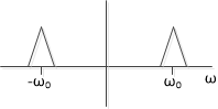
Figure 1.  Spectrum of a Bandpass Signal

Since Hilbert Transformers are frequently used with modulated signals, we start with a definition of bandpass modulation from Sklar [1]:

Bandpass modulation (either analog or digital) is the process by which an information signal is converted to a sinusoidal waveform …  The sinusoid has just three features that can be used to distinguish it from other sinusoids:  amplitude, frequency, and phase.  Thus bandpass modulation can be defined as the process whereby the amplitude, frequency, or phase of an RF carrier, or a combination of them, is varied in accordance with the information to be transmitted.

A modulated signal x(t) can be written as:

$$x(t)=A(t)cos(\omega_0t + \theta(t)) \qquad(1)$$

where A(t) is amplitude (also referred to as the signal envelope), ω₀ is carrier frequency, and θ is carrier phase.  An equivalent expression is:

$$x(t)=A(t)cos(\phi(t)) \qquad(2)$$

where $\phi(t)=\omega_0t+\theta(t)$.  We can also represent the signal using a complex exponential:

$$x(t)= A(t)Re\{cos\phi+jsin\phi\} \qquad$$

$$\qquad=Re\{x_r+jx_i\}\qquad\qquad(4)$$

Where $x_r=A(t)cos\phi$  and  $x_i=A(t)sin\phi$.  Figure 2 shows the modulated signal as a vector in the complex plane.

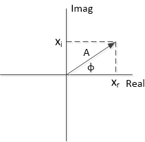
Figure 2.  Modulated Signal in the complex plane.

The Hilbert Transformer

When demodulating x(t), our go-to first step is normally quadrature down-conversion.  This approach allows us to apply lowpass filters to the I and Q channels, which is an important advantage.  Here we’ll take a different approach that does not replace quadrature conversion, but has its own particular uses.  What if we had a device that could generate x_r and x_i of Equation 4 directly from x(t), without down-conversion?  This would be an alternative first step in demodulation (or other processing) of x(t), and it is what the Hilbert Transformer provides.

We’ll start by considering continuous-time signals.  Figure 3 shows what we are trying to do.  We are looking for a filter h(t) with:

$$input= x_r(t)=A(t)cos(\omega_0t+\theta(t))\qquad\qquad$$

$$output= x_i(t)=A(t)sin(\omega_0t+\theta(t))\qquad(5)$$

We then form the complex signal:

$$x_c(t)= x_r(t)+jx_i(t)\qquad(6)$$

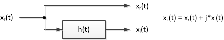
Figure 3.  Hilbert Transformer

Suppose x_r is an unmodulated cosine with A(t)= 1.  The Fourier Transform of a cosine is shown in the top of Figure 4.  This spectrum is given by [2]:

$$X_r(\omega)=\pi[\delta(\omega+\omega_0)+\delta(\omega-\omega_0)]\qquad(7)$$

Our goal is to obtain the sine spectrum shown in the bottom of Figure 4 for any value of ω₀:

$$X_i(\omega)=H(\omega)X_r(\omega)=j\pi[\delta(\omega+\omega_0)-\delta(\omega-\omega_0)]\qquad(8)$$

where the transfer function H(ω) is the Fourier Transform of h(t).  The H(ω) needed to create X_i(ω) is simply:

$$H(\omega)=\frac{X_i(\omega)}{X_r(\omega)}=\quad j,\;\omega<0$$

$$\qquad\qquad\qquad\qquad\qquad\qquad\qquad -j,\;\omega\ge0\qquad\qquad(9)$$

This rather peculiar-looking transfer function is shown in the middle of Figure 4.  We see that H(ω) provides a +90 degree shift for ω < 0, and a -90 degree shift for ω > 0 (recall that j = e^jπ/2).

Once we know the impulse response h(t) that corresponds to H(ω), we can use it to find x_i for any modulated bandpass signal.  We can then compute A(t) and φ(t) with reference to Figure 2:

$$ A(t)=\sqrt{x_r^2+x_i^2}\qquad(10)$$

$$ \phi(t)=tan^{-1}(x_i/x_r)\qquad(11)$$

Equation 10 represents amplitude demodulation, while Equation 11 represents phase demodulation.  The time derivative of Equation 11 provides dφ/dt, i.e., frequency demodulation.

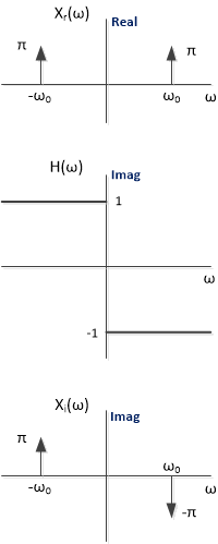
Figure 4.  Top: Cosine spectrum X_r(ω).  Middle: Hilbert Transformer Transfer Function H(ω).  Bottom: Sine Spectrum X_i(ω) = X_r(ω)* H(ω).

Hilbert Transformer Impulse Response and Structure

The middle plot of Figure 4 shows the frequency response of an ideal continuous-time Hilbert Transformer.  Figure 5 shows the frequency response of an ideal discrete-time Hilbert transformer, where f_s is the sample frequency.  We can find the impulse response using the inverse Fourier Transform [3]:

$$h(n)=\frac{2}{n\pi}sin^2(n\pi /2),\quad -\infty < n < \infty \qquad(12)$$

This impulse response is plotted in Figure 6.  We make the following observations:  First, h(n) is odd-symmetric, which follows from the fact that H(f) is pure imaginary.  Second, the sample values are proportional to 1/n, and every other sample of h(n) is zero.  Third, h(n) has infinite length, and it begins before n = 0 (it is non-causal).

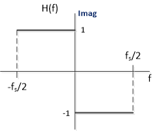
Figure 5.  Ideal Discrete-time Hilbert Transformer Frequency Response H(f).

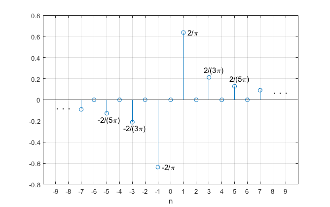
Figure 6.  Ideal Discrete-time Hilbert Transformer Impulse Response.

So how do we design a practical Hilbert Transformer?  There are a few approaches.  One way is to truncate the ideal impulse response and then apply a window function.  Another approach, which we’ll discuss in Part 2, uses a half-band filter as the starting point of the design.  Suppose we use one of these approaches to design a 7-tap Hilbert Transformer.  The coefficients can then be written as:

b = [b_-3 0 b_-1 0 b₁ 0 b₃]

where, due to the odd symmetry, b₁ = -b_-1 and b₃ = -b_-3.  We note that the number of taps is odd, and every other tap value is zero.  The delay of this filter is (ntaps-1)/2 = 3 samples, as opposed to a delay of zero for the non-causal filter.  Because of the non-zero delay, we cannot directly implement the block diagram of Figure 3, in which the x_r output is identical to the input.  The Hilbert Transformer can instead be implemented using the FIR structure in Figure 7, where we take x_r from the output of the center tap to match the 3-sample delay of x_I.  We have also labeled the input x (no subscript), to distinguish it from x_r.

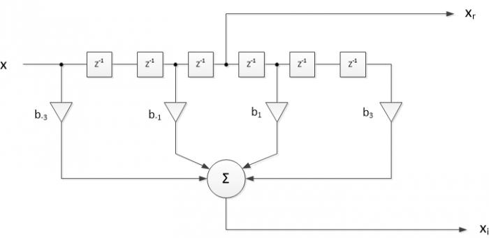
Figure 7.  Discrete-time Hilbert Transformer with ntaps = 7.

Hilbert Transformer Output Spectrum

In Equation 6, we defined the Hilbert Transformer’s output x_c as complex, which has an effect on its output spectrum.  To examine the spectrum, consider the special case where continuous-time x_r(t) is an even-symmetry modulated signal, with carrier frequency ω₀.  Then the spectrum X_r(ω) is real and even, as shown in the top of Figure 8.  Applying this signal to the Hilbert Transformer, we get the pure imaginary spectrum X_i(ω), as shown in the middle plot.  We then multiply by j, to get jX_i in the bottom plot, which is pure real (recall j² = -1).  Forming X_c = X_r + jX_i, the components centered at - ω₀ cancel, and we get the spectrum shown on the right.  We call a signal with a one-sided spectrum an analytic signal.  Note also that the level of the analytic signal’s spectrum is twice that of each component of the real signal’s spectrum.

Now we’ll show that the output spectrum is analytic for a general input signal.  The frequency response of the Hilbert Transformer’s complex output is:

$$G(\omega)=\frac{X_r+jX_i}{X_r}\qquad(13)$$

or,

$$G(\omega)=1+jH(\omega)\qquad(14)$$

Then, from Equation 9,

$$G(\omega)= 0,\quad \omega < 0$$

$$\qquad\qquad\qquad\quad 2,\quad \omega \ge 0 \qquad (15) $$

G(ω), which is pure real, is plotted in Figure 9.  The response is zero for ω < 0, and thus the output is analytic for any input signal.  We again see a factor of two gain for ω > 0.  Note that while the transfer function G(ω) is pure real, the output signal x_c(t) is complex.

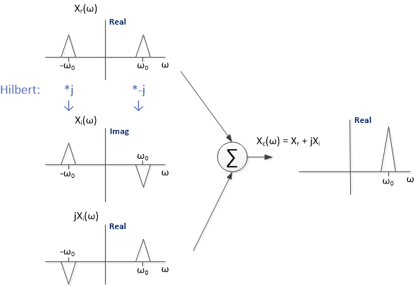
Figure 8.  Spectrum of X_c(ω) for an even-symmetry bandpass input signal.

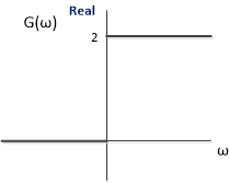
Figure 9.  Frequency Response of Hilbert Transformer complex output.

Example 1.  Sanity Check

If the Hilbert Transformer really works, we should be able to use a Matlab model of it to create quadrature sinusoids (cosine/sine) from a sinusoidal input of arbitrary frequency.  But first, we’ll compute the Hilbert Transformer’s frequency response.  We note that H(z) of the Hilbert Transformer is defined with respect to the center tap, so:

$$H(z)=\frac{H_{FIR}(z)}{z^{-K}}\qquad (16)$$

where H_FIR(z) is the causal transfer function of the Hilbert Transformer and K samples is the delay of the center tap.

For our model, we’ll use the Hilbert Transformer coefficients listed below (I will discuss Hilbert Transformer design in Part 2).  The length of the filter is 19 taps.  H(f) is calculated from the coefficients b_hilb and b_ct as shown, where b_ct is the impulse response of the center tap and f_s = 200 Hz is the sample frequency.

    b_hilb= [-4 0 -21 0 -64 0 -170 0 -634 0 634 0 170 0 64 0 21 0 4]/1024;
    b_ct= [0 0 0 0 0 0 0 0 0 1 0 0 0 0 0 0 0 0 0];
    N= 1024;                % number of samples/fft length
    fs= 200;                % Hz sample frequency
    % HT freq response
    [H,f]= freqz(b_hilb,b_ct,N,fs,'whole');

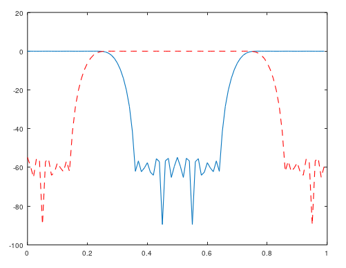
H(f) is plotted over 0 to f_s in Figure 10, along with the ideal response.  Note that the frequency range f_s/2 to f_s (100 – 200 Hz) of the discrete-frequency response corresponds to f < 0 of the continuous response.  We see that the transfer function of a practical Hilbert Transformer departs from the ideal near 0 and f_s/2.  There is also some ripple in the passband.  In this case, the response is reasonably accurate over f = 19 to 81 Hz.  Although the transfer function is not ideal, it is nevertheless pure imaginary.  This follows from the odd symmetry of the coefficients.

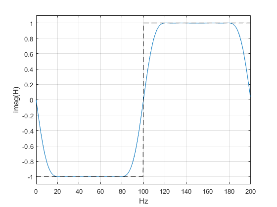
Figure 10.  19-tap Hilbert Transformer Frequency Response, with ideal response (dashed), f_s = 200 Hz.

Now we’ll generate a cosine at 20 Hz, and filter it with the Hilbert Transformer, using the code listed below.  One cycle of the outputs x_r and x_i are plotted in Figure 11, where you can see the phase difference of 90 degrees.

    fs= 200;                % Hz sample frequency
    Ts= 1/fs;               % s sample time
    f0= 20;                 % Hz frequency of input cosine
    N= 64;                  %    number of samples
    n= 0:N-1;               % time index
    x= cos(2*pi*f0*n*Ts);   % input cosine
    % Filter x using Hilbert Transformer
    x_r= conv(x,b_ct);      % x_r is output of center tap
    x_i= conv(x,b_hilb);
    plot([x_r' x_i'],'.-','markersize',9),grid
    axis([30 40 -1 1])

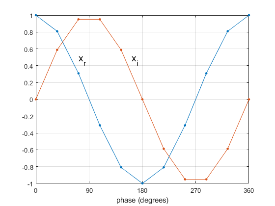
Figure 11.  One cycle of Hilbert Transformer outputs for input sinusoid at 20 Hz and f_s = 200 Hz.

We can also compare the spectra of the input and complex output of the Hilbert Transformer.  We’ll use the same code as above to generate x_r and x_i, but with changes to the input cosine’s frequency and number of samples:

                    f0= 27;            % Hz frequency of input cosine
                    N= 512;            %    number of samples

Next, we form the complex output x_c.  Then we apply a window function [4] to x and x_c before performing an FFT:

    x_c= x_r + j*x_i;                % complex output signal
    x_c= x_c(10:end-9);              % limit length to N
    % window x and x_c for fft
    win= kaiser(N,8)'/((N+1)/2);     % Kaiser window function
    x_win= win.*x;
    x_c_win= win.*x_c;
    % spectra of real input and complex output
    X= fft(x_win,N);
    Xc= fft(x_c_win,N);
    X_dB= 20*log10(abs(X));
    Xc_dB= 20*log10(abs(Xc));
    f= n*fs/N;                      % Hz discrete frequency

The resulting spectra are shown in Figure 12.  The output spectrum is approximately analytic.  There is a remaining image component at 173 Hz that is about 60 dB below the desired component.  We also note that, as expected, the magnitude of the analytic signal x_c at 27 Hz is 6 dB higher than the input signal components (factor of 2).

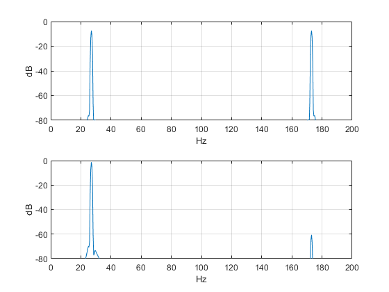
Figure 12.  Top: Spectrum of Hilbert Transformer input, f₀ = 27 Hz and f_s = 200 Hz.

Bottom: Spectrum of Hilbert Transformer complex output x_c. 

Example 2.  Calculating Image Attenuation of a Hilbert Transformer

In figure 12, we see that the Hilbert Transformer image at 173 Hz is attenuated about 60 dB relative to the desired signal at 27 Hz.  Can we find the image attenuation vs. frequency over the entire band from f_s/2 to f_s?  Indeed we can:  it can be read from a plot of the frequency response of the Hilbert Transformer’s complex output.  From Equation 14, this is:

$$G(f)= 1+jH(f)$$

Where f is discrete frequency.  We can compute H(f) from our Hilbert Transformer coefficients, and then use H(f) to find G(f).

The appendix lists a Matlab function called hilbert_image for calculating and plotting the response of a Hilbert Transformer’s complex output.  For the filter of Example 1, we plot the response using hilbert_image as follows:

    fs= 200;              % Hz sample frequency
    nfft= 512;            %    number of points in freq. response
    b_hilb= [-4 0 -21 0 -64 0 -170 0 -634 0 634 0 170 0 64 0 21 0 4]/1024;
    hilbert_image(b_hilb,nfft,fs);

The Matlab function’s output is shown in Figure 13, where H(f) (top) and G(f) (middle) are plotted using linear amplitude scales.  The response relative to the passband of G is G_rel = G/2, which is plotted using a dB amplitude scale (bottom).  Again, the frequency range f_s/2 to f_s (100 – 200 Hz) of the discrete-frequency response corresponds to f < 0 of the continuous response.  We see from the G_rel plot that the response at 173 Hz is about -60 dB, as expected.

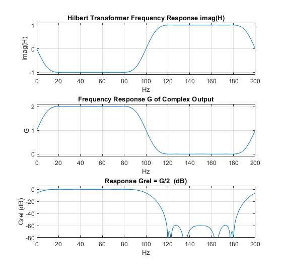
Figure 13.  Top: Hilbert Transformer Frequency Response imag[H(f)], f_s = 200 Hz.

Middle: Frequency Response of Complex Output, G(f).

Bottom: Frequency Response of Complex Output, G_rel = G(f)/2, in dB.

Example 3.  Amplitude Demodulation

An amplitude-modulated signal can be written as:

$$x(t)= M[1+m(t)]cos(\omega_0t)= A(t)cos(\omega_0t)\qquad(17)$$

Where ω₀ is the carrier frequency, M is amplitude of the unmodulated carrier, and m(t) is the modulating signal.  If we apply x(t) to a Hilbert Transformer, we can find the modulation envelope A(t) by using Equation 10:

$$ A(t)=\sqrt{x_r^2+x_i^2}$$

The block diagram of a Hilbert AM envelope detector is shown in Figure 14.  The (analog or digital) bandpass filter is needed if noise or adjacent signals are present.

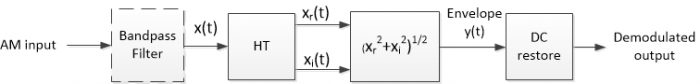
Figure 14.  Envelope detector using the Hilbert Transformer.

Now we’ll create a Matlab model of an AM demodulator.  We’ll use the same Hilbert Transformer coefficients used in the previous examples:

    b_hilb= [-4 0 -21 0 -64 0 -170 0 -634 0 634 0 170 0 64 0 21 0 4]/1024;
    b_ct= [0 0 0 0 0 0 0 0 0 1 0 0 0 0 0 0 0 0 0];

Next we’ll create an AM signal with sinusoidal modulation.  Let carrier frequency be 22 Hz, modulation frequency be 3 Hz, and sample frequency be 200 Hz.

    N= 512;                      % number of samples
    fs= 200;                     % Hz sample frequency
    n= 0:N-1;                    % sample index
    Ts= 1/fs;                    % s sample time
    fc= 22;                      % Hz carrier frequency
    fm= 3;                       % Hz modulating frequency
    carr= cos(2*pi*fc*n*Ts);     % carrier
    m= .9*cos(2*pi*fm*n*Ts);     % modulating signal
    A= 1 + m;                    % envelope
    x= A.*carr;                  % modulated signal

To demodulate x, we perform the operations shown in Figure 14:

    % Filter x using Hilbert Transformer
    x_r= conv(x,b_ct);
    x_i= conv(x,b_hilb);
    % demodulation
    y= sqrt(x_r.^2 + x_i.^2);     % y ~= A

The dc restorer is a first-order high-pass IIR filter with coefficients as shown [5]:

    b= [1 -1];
    a= [1 -31/32];
    m_rx= filter(b,a,y);    % m_rx ~= m

The modulated signal x and the demodulated envelope y are plotted in the top of Figure 2, and the recovered signal m_rx is shown in the bottom.  Finally, there are several numerical methods to compute $\sqrt{x_r^2+x_i^2}$ .  An efficient method of moderate accuracy is presented in [6].  Another option is the CoRDiC algorithm [7]. 

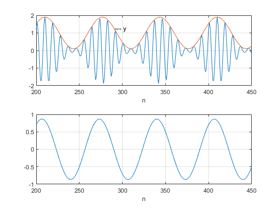
Figure 15.  AM Demodulator.  Top: Modulated signal and detected envelope y(t).

Bottom: DC-restored output.

Example 4.  Phase or Frequency Shifter

I described Hilbert-based phase and frequency shifters in an earlier post [8].  The Hilbert Transformer, with its analytic spectrum, is particularly suited here.  Note:  the Hilbert Transformer design in this post uses the window method.  In Part 2 of this article, I’ll describe a different design method that uses half-band filter coefficients as the starting point of the design.

Example 5.  Phase Detector for a Phase-Locked Loop

This is another application described in an earlier post [9].

For the Appendix, see the PDF version of this article.

References

1.  Sklar, Bernard, Digital Communications, Prentice Hall, 1988, p 127.

2.  Hayt, William H., et. al., Engineering Circuit Analysis, 8^th Ed., McGraw Hill, 2012, p 765-766.

3.  Lyons, Richard G., Understanding Digital Signal Processing, 3rd Ed., Pearson, 2011, p 487-488.

4.  Robertson, Neil, “The Discrete Fourier Transform and the Need for Window Functions”, DSPRelated.com, Nov. 15, 2021, https://www.dsprelated.com/showarticle/1433.php

5.  Lyons, section 13.23.

6.  Lyons, section 13.2.

7.  Rice, Michael, Digital Communications, a Discrete-Time Approach, Pearson, 2009, section 9.4.

8.  Robertson, Neil, “Phase or Frequency Shifter Using a Hilbert Transformer”, DSPRelated.com, March 25, 2018, https://www.dsprelated.com/showarticle/1147.php

9.  Robertson, Neil, “Digital PLL’s Part 3 – Phase Lock an NCO to an External Clock”, DSPRelated.com, May 27, 2018, https://www.dsprelated.com/showarticle/1177.php

Neil Robertson       November, 2022

Sign in