


Computing Fixed-Point Square Roots and Their Reciprocals Using Goldschmidt Algorithm
Introduction
A well known algorithm for computing square roots by iteration is provided by the Newton-Raphson Algorithm. The algorithm determines the square root using iteration until the root has been determined to some user-defined level of accuracy. The method is easily derived. First, describe a number in terms of its square root:
$$ a = y ^ {2} ,$$
where $y = \sqrt{a}$. The value of the $\sqrt{a}$ can be written as $y = y_0 + \epsilon$, where $y_0$ is the value of the square root and $\epsilon$ is the error in the square root. Thus,
$$ a = y ^ {2} = \left ( y_0 + \epsilon \right ) ^ {2} = y_0^2 + 2{\epsilon}{y_0} + {\epsilon}^{2}.$$
Ideally, we want to know that whatever value we compute for the square root is close to the actual value. In other words, the error, $\epsilon$, should be trending toward zero when the algorithm terminates. Therefore,
$$a = y_0^2 + 2{\epsilon}{y_0}$$
and
$$\epsilon = \frac{a - y_0^2}{2y_0}$$.
Substituting $\epsilon$ into $y = y_0 + \epsilon$ yields:
$$y = \frac{1}{2}\left (\frac{a}{y_0}+y_0\right).$$
This result can be represented as a recursion:
$$y_i= \frac{1}{2}\left (\frac{a}{y_{i-1}}+y_{i-1}\right).$$
To achieve quadratic convergence on the square root, an initial estimate of the root, $y_0$, is required. An estimate too far from the true root will cause convergence to be linear instead of quadratic. In other words, if the initial estimate of the root, $y_0$,is much less than or greater than the root, then each iteration approaches the root linearly according to:
$$y_i = \frac{y_{i-1}}{2}.$$
Quadratic convergence returns to the recursion once the approximation of the root, $y_i$, is in the vicinity of the real root. Therefore, a good initial estimate of the root is required.
Another feature of the Newton-Raphson square root algorithm is that each iteration requires a division to be performed. In terms of computer arithmetic, division is generally far slower than multiplication except when these operations can be implemented as right shift and left shift operations, respectively.
Estimating $y_0$ for Floating Point Implementations
There are several approaches used to choose $y_0$.
For floating point numbers, one approach is to break apart the
floating point format, i.e. into its exponent and mantissa
components. The estimate of the square root is obtained by simply
manipulating the exponent and putting the components back together
again. This approach works for floating point representations because
the mantissa represents a constrained range of numbers: $0.5$ to $1.0$.
The floating point exponent allows a much larger set of numbers.
Thus,
$$\sqrt{a{2}^{30}}=\sqrt{a}{2}^{15}.$$
Since the mantissa is generally a number between $0.5$ and $1.0$, the
square root of the mantissa lies between $\sqrt{2}/2$ and $1.0$. If the square root
of the mantissa is assumed to be $1.0$, the estimate of the square root
is defined as magnitude of the exponent divided by $2$. The
additional iterations that may result from using this value for $y_0$ are generally low. So this approach,
although not optimal, represents a good, robust approach that is easy to implement and does not significantly impact performance.
Another approach to determine the estimate of the square root is to use tables, with the objective to refine the initial estimate and minimize the number of iterations required to converge to the root. This is the approach used for many square root implementations in many floating point processors. On an historical note, an incompletely specified table was the source of the infamous FDIV error in the Intel Pentium processor.
Fixed-Point Goldschmidt $\sqrt{S}$ and $1/\sqrt{S}$ Algorithm Description
The introduction section provides a derivation of a square root algorithm based on the algorithm of Newton and Raphson. In addition, it discusses an approach for estimating the initial value of the square root for floating point values so that quadratic, rather than linear, convergence to the root can be achieved. For the target application, 32-bit fixed-point numbers are used instead of floating point numbers. (Note: the primary reason for using the 32-bit fixed-point representation is that the algorithm is implemented to support a motion controller embedded in an FPGA's programmable logic rather than in an FPGA using an embedded soft-core microprocessor.)
The Goldschmidt square root algorithm powers the square root operations found in some current floating-point processors. It can be used to compute square roots and inverse square roots for fixed-point processors. This section will describe the algorithm as it applies to fixed-point representations. (Note: the implementation of the algorithm for floating-point representations can be easily determined from the discussion that follows.)
Initial Fixed-Point Square Root Estimate, $y_0$
The approach required to estimate the initial starting value of the root for fixed-point representations is similar to that used for floating-point representations. However, the fact that fixed-point representations provide both an integer and a fractional component complicates how the estimate is computed. The primary factor complicating the estimation of the initial square root value for fixed-point representation is that the algorithm simultaneously computes that square root and the inverse square root. The inverse square root of a fractional-only fixed-point value may have a fixed-point integer component that exceeds the fixed-point representation's integer component. (Note: for a fully general purpose algorithm, changing the decimal point location in the fixed-point representation would be a requirement. However, for the target application, the range of fixed-point values to which the algorithm is applied can be limited in a manner that avoids the need to float the decimal point of the fixed-point representation.)
The approach taken for floating point numbers can be adapted to
support fixed-point numbers, because the mantissa of floating-point values represents a
limited range, and the magnitude of the floating-point number's exponent divided by two is a
good initial estimate of the square root. Therefore, an estimate of the fixed-points number square root based on the
most significant bit of the fixed-point number will yield a good
initial estimate of the square root for fixed-point numbers. The most
significant number of the fixed-point number is equivalent to the
following:
$$\mathtt{msb}(S)=m=\lfloor{\log_2{S}}\rfloor-b_{fraction}$$
where $S$ is a 2's complement 32-bit fixed-point value with a 16-bit fractional part, i.e. $b=16$. For this specific format, for which we will derive the Goldschmidt Square Root Algorithm, the positive range of the representation is $0$ to $32767.99999$. Thus, $m$ ranges from $-12$ to $15$, and the estimate of the square root, $y_0$ is provided by the following equation:
$$y_0 = \left(\sqrt{S}\right)_{est} = \sqrt{2^m}2^b$$
For example, the square root of $32767.99999$ when represented as a 32-bit, fixed-point value with a 16-bit fractional part, i..e FP32B16, is not $\sqrt{2,147,483,647}$. Instead, the correct estimate is computed as:
$$m=\mathtt{msb}(2,147,483,647)-b_{fraction}$$
$$m=\lfloor{\log_2{2,147,483,647}}\rfloor-b_{fraction}$$
$$m=30-16=14$$
and
$$y_0 = \left(\sqrt{S}\right)_{est} = \sqrt{2^m}2^b=\sqrt{2^{14}}2^{16} = 8,388,608$$
Thus, the initial estimate of the root, $y_0$, is $128$, and the real root of $\sqrt{32767.99999}$ is $181.01934$.
Since the square root is required in real-time in the target application, it is desired that the number of
iterations required to converge on the square root is the same at
both edges of each region, i.e. for each value of the $\mathtt{msb}(S)$
function. In other words, the number of iterations needed to compute
the square root using the Goldschmidt fixed-point algorithm should be the same at each boundary:
$$\mathtt{iter}\left(\sqrt{2^{m}}2^{16}\right) = \mathtt{iter}\left(\sqrt{2^{m+1}}2^{16}\right)$$
Setting the number of iterations required for convergence constant at both boundaries, allows the algorithm to be implemented using a fixed number of iterations and removes the requirement for a convergence test to terminate the algorithm. However, the shape of the square root function means that it is very unlikely that the error in the estimate will be the same at both ends of the range represented by each $\mathtt{msb}(S)$. A multiplicative adjustment applied to each segment may be able to make the number of iterations required for convergence the same at each extreme of a segment, and the same for all segments in the range of values for which the algorithm will be required to calculate the square root and inverse square root. Such a value can be found, so the previous equation can be written as:
$$\mathtt{iter}\left(\sqrt{2^{m}}2^{16}N_{adj}\right) = \mathtt{iter}\left(\sqrt{2^{m+1}}2^{16}N_{adj}\right)$$
The value of $N_{adj}$ that makes the number of iterations the same for each boundary of a segment can be found using the "What If" function in Microsoft Excel. Thus, in addition to the $\mathtt{msb}()$ function, a small pre-calculated table for the 27 segments for $m = \left[-12,\ldots,15\right)$ is all that is required to estimate the initial value of the square root for the Goldschmidt square root algorithm. (Note: for these values of $m$, a value for $N_{adj}$ of $1.23898296208219$ was found to make the number of iterations required for convergence to be equal to $5$. In the FP32B16 fixed-point representation, for values less than 4096, i.e. $m=-12$, some suitable value for the square root and inverse square root can be returned.)
Floating-Point Goldschmidt $\sqrt{S}$ and $1/\sqrt{S}$ Algorithm Description
There are two algorithms for the Goldschmidt computing $\sqrt{S}$ and $1/\sqrt{S}$. These algorithms will be defined in the following two subsections.
Floating-Point Goldschmidt $\sqrt{S}$ and $1/\sqrt{S}$ Algorithm #1
Algorithm #1 uses four variables: $b$, $Y$, $x$, and $y$. The initial values of these variables are initialized in the following manner:
$$b_0 = S$$
$$Y_0 = \left(\frac{1}{\sqrt{S}}\right)_{est}$$
$$x_0 = SY_0$$
$$y_0 = Y_0$$
The algorithm is performed by evaluating the following recursion equations:
$$b_i = b_{i-1}Y^2_{i-1}$$
$$Y_i = \frac{3 - b_i}{2}$$
$$x_i = x_{i-1}Y_i$$
$$y_i = y_{i-1}Y_i$$
The algorithm has converged on the root and can be terminated when $b_i \le 1 - \epsilon$, where $\epsilon$ is a predetermined error bound, or after a pre-determined number of iterations. The $\sqrt{S}$ and $1/\sqrt{S}$ are given by:
$$\sqrt{S} = x_i$$
and
$$\frac{1}{\sqrt{S}} = y_i$$
Floating-Point Goldschmidt $\sqrt{S}$ and $1/\sqrt{S}$ Algorithm #2
Algorithm #2 uses three variables: $r$, $x$, and $h$. The initial values of these variables are initialized in the following manner:
$$x_0 = S\left(\frac{1}{\sqrt{S}}\right)_{est}$$
$$h_0 = \frac{1}{2}\left(\frac{1}{\sqrt{S}}\right)_{est}$$
$$r_0 = \frac{1 - 2 x_0 h_0}{2}$$
The algorithm is performed by evaluating the following recursion equations:
$$x_i = x_{i-1}\left(1+r_{i-1}\right)$$
$$h_i = h_{i-1}\left(1+r_{i-1}\right)$$
$$r_i = \frac{1 - 2 x_i h_i}{2}$$
The algorithm has converged on the root and can be terminated when $r_i \le \epsilon$, where $\epsilon$ is a predetermined error bound, or after a pre-determined number of iterations. The $\sqrt{S}$ and $1/\sqrt{S}$ are given by:
$$\sqrt{S} = x_i$$
and
$$1/\sqrt{S} = 2h_i$$
Selection of Algorithm to Implement in Fixed-Point
Testing of these two algorithms using Excel demonstrated that Algorithm #1 appeared to be more consistent with respect to the termination condition. Even though a fixed number of iterations, i.e. 6 or initialization plus five more cycles, was the goal, Algorithm #1 appeared to provide a more robust way to terminate. Therefore, Algorithm #1 was selected for implementation in fixed-point.
Fixed-Point Implementation of Goldschmidt Algorithm #1
Define $B = 2^{b_{fraction}}$ as the base for the decimal point in the selected fixed-point representation. For the target application, and for the previous development, $B$ is $2^{16}$, or $65536$. With B defined, it is possible to define Goldschmidt algorithm #1 to support fixed-point numbers. The initialization equations are defined as follows, where $S_{FP}$ is the fixed-point value to which the algorithm will be applied:
$$m = \mathtt{msb}(S_{FP})$$
$$b_0 = S_{FP}$$
$$Y_0 = Y_{est}[m]$$
$$x_0 = \frac{S_{FP}Y_0}{B}$$
$$y_0 = Y_0$$
The solution is performed by iterating the following recursion equations:
$$b_i = \frac{b_{i-1}Y_{i-1}}{B}\frac{Y_{i-1}}{B} = \frac{b_{i-1}Y^2_{i-1}}{B^2}$$
$$Y_i = \frac{3B-b_i}{2}$$
$$x_i = \frac{x_{i-1}Y_i}{B}$$
$$y_i = \frac{y_{i-1}Y_i}{B}$$
The algorithm has converged when $b_i \le B(1-\epsilon)$, or when a pre-determined number of iterations have been performed. The results are:
$$\sqrt{S_{FP}} = x_i$$
$$\frac{1}{\sqrt{S_{FP}}} = y_i$$
(Note: when implementing fixed-point arithmetic, the upper half of the double length product is generally the desired result. When multiplying fixed-point numbers with varying numbers of fractional bits, a normalization step is required following the computation of any fixed-point products. That normalization step usually involves shifting the double length product right / left as necessary to ensure the correct number of fractional bits are preserved and written to the result register. In the description of the algorithm in this article, the representation is maintained as FP32B16, i.e. a signed 32-bit fixed-point number with 16 fractional bits. Thus, after each product, the double length result has to be right shifted by the number of fractional bits in the representation.
In the fixed-point arithmetic unit implemented for the target application, left/right shifts of the double length product are provided by a single cycle barrel shifter at the output of the multiplier. This means that the arithmetic right shift operation shown in the equations above are free. Similarly, operations like scaling by powers of 2 are also free.
Finally, for the target application, the fixed-point arithmetic was performed using 32-bit signed values. The double length fixed-point product was generated using a 4-bits at a time Booth multiplier rather than a multiplier constructed from the built-in 18-bit multiplier-accumulators available in the target application's FPGA. The custom-designed, Booth multiplier does not deliver single cycle performance, or even 4 cycle performance. In fact, it requires 11 cycles to compute the product (10 for the multiplier and 1 for the barrel shifter) since in the target application both the ALU and the multiplier are actually implemented as 40-bit wide functions in order to provide guard bits on both ends in order to support chained operations and improved rounding / truncation of intermediate results. Taken all together, the Booth multiplier is slightly slower and uses fewer resources than a multiplier built with the built-in hardware multipliers of the target FPGA for a similar numerical format.)
Generating $Y_{est}[m]$ Table
Like the floating-point algorithms, the fixed-point algorithm is dependent on a “good” estimate of $1/\sqrt{S_{FP}}$ to limit the number of iterations needed for convergence. The square root estimate previously described is a good starting point, and simply needs to be inverted to provide the necessary estimated for the fixed-point Goldschmidt algorithm. A table containing the pre-computed estimates for the fixed-point inverse square roots required for the fixed-point Goldschmidt algorithm can be generated as follows:
$$Y_{est}[m] = \frac{B}{\sqrt{2^m}N_{adj}}, \{m: -12\ldots+15\}$$
where $N_{adj} = 1.238982962$. With the inverse square root provided by the estimate provided by $Y_{est}[m]$, the algorithm converges in five iterations. (Note: interestingly, if the estimate provided for the fixed-point algorithm is used for the floating-point algorithm, convergence of the floating point algorithm is also 5 iterations.)
Summary
The Fixed-Point Goldschmidt $\sqrt{S_{FP}}$ and $1/\sqrt{S_{FP}}$ algorithm provides an effective way to solve for the square root and inverse of the square root of a number. The solutions provided by the algorithm are required to implement solutions to the Law of Cosines, which is required to convert the control variable from angular rate about the hinge into linear extension rate of the actuators in the target application. It also provides the benefit that it can be easily extended to support division if that mathematical operation becomes necessary.


- Comments
- Write a Comment Select to add a comment

Hi Michael Morris.
Near the first part of your blog you have the equation:
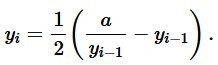
I think the minus sign in that equation should be a plus sign.

Rick:
Thanks very much for your comment. You're correct. I mistranslated that equation from out of my original paper. I will update the post.
Michael A. Morris
Hi Michael. Just so you know, if I had a dollar for every time I made a similar "sign" error I'd be able to buy a new set of tires for my car.
The topic of you blog is an important one. I look forward to reading the remainder of your blog.
Rick:
Thanks for your response. I understand completely, and I really appreciate you taking the time to comment about the sign error. I skipped some of the steps in the derivation that I have in my original paper, and I must have lost my place in the transcription.
I don't have strong math skills, and it's important to be able to assume that the the final equations of an significant derivations are correct. So I really appreciate you pointing out the sign error so that others with similar skills are not tripped up by it if they wanted to test out that simple formula for the square root.
Once again thanks for the heads up. It also gave me the opportunity to correct some of the text and add some missing words and correct some verb tenses. Even after reviewing it several times before posting it, several errors appeared in the final. You at least pointed out a significant error, and not a grammar or spelling error. :) I am sure that there probably other errors remaining.
Michael A. Morris
In algorithm #2 the error bound comparison uses b_i <= epsilon but b_i is not defined for algorithm #2. Which of the defined values should be used? I'd assume r_i would be the correct value to used.
Corrected as suggested. Thank you.

Thanks for the comment.

Nice article. I'm familiar with this approach -- in a former company, we used it in a TI TMS320F24xx motor control DSP around 1999 or 2000 -- but never heard it mentioned as "Goldschmidt's Algorithm" before; we always thought it was just Newton's method for inverse square root with just addition/multiplication. (which it is, but I guess there are some specific flourishes that add onto the base Newton's method.)
I don't remember where I learned about it from, though. (I thought it had been Numerical Recipes, but I don't see it anywhere. Maybe Knuth TAOCP v2?)
Here's a paper that mentions it and cites Goldschmidt's M.S. 1964 thesis: https://citeseerx.ist.psu.edu/viewdoc/download?doi...
To post reply to a comment, click on the 'reply' button attached to each comment. To post a new comment (not a reply to a comment) check out the 'Write a Comment' tab at the top of the comments.
Please login (on the right) if you already have an account on this platform.
Otherwise, please use this form to register (free) an join one of the largest online community for Electrical/Embedded/DSP/FPGA/ML engineers: