A Simplified Matlab Function for Power Spectral Density

In an earlier post [1], I showed how to compute power spectral density (PSD) of a discrete-time signal using the Matlab function pwelch [2].  Pwelch is a useful function because it gives the correct output, and it has the option to average multiple Discrete Fourier Transforms (DFTs).  However, a typical function call has five arguments, and it can be hard to remember how to set them all and how they default.

In this post, I create a simplified PSD function by putting a wrapper on pwelch that sets some parameters and converts the output units from W/Hz to dBW/bin.  The function is named psd_simple.m, and its code is listed in the appendix.

The function is called as follows:

    [PdB,f]= psd_simple(x,nfft,fs);

The input arguments are:

x          input signal vector

nfft       number of points in the DFT.

fs         sample rate in Hz

Let length(x) = N.  Setting nfft = N results in a PSD without DFT averaging.  To use DFT averaging, set nfft to a fraction of N (e.g. N/8).  This causes the function to use windowed segments of x of length nfft as inputs to the DFT.  The |X(k)|² of the multiple DFT’s are then averaged.

The output arguments are:

         PdB       PSD in dBW/bin

         f             vector of frequency values from 0 to fs/2 (for x real)

For real x, the length of the output vectors is nfft/2 + 1 when nfft is even.  For example, if nfft = 1024, PdB and f contain 513 samples.  PdB has units of dBW/bin when x has units of volts and load resistance is one ohm. (This is different from the output pxx of pwelch, which has units of W/Hz).

psd_simple uses a Kaiser window function [3,4] with beta = 7.  For DFT averaging, the segment overlap is set to nfft/2.

Why use dBW/bin?

Computing the PSD in dBW/bin allows reading the power of a sinewave’s spectral component directly from the PSD plot.  The power is constant vs nfft.

Example 1.

This example uses the same signal as my post on pwelch.  The signal x consists of a sine wave plus Gaussian noise.  Here is the code to generate x, where the sine frequency is 500 Hz and the sample rate is 4000 Hz:

    fs= 4000;            % Hz sample rate
    Ts= 1/fs;
    f0= 500;             % Hz sine frequency
    A= sqrt(2);          % V sine amplitude for P= 1 W into 1 ohm.
    N= 1024;             % number of time samples
    n= 0:N-1;            % time index
    x= A*sin(2*pi*f0*n*Ts) + 0.1*randn(1,N);

The power of the sine wave into a 1-ohm load is A²/2 = 1 watt.  To compute the spectrum without DFT averaging, we use:

    nfft= N;
    [PdB,f]= psd_simple(x,nfft,fs);

The resulting PSD is plotted in Figure 1.  Since the units of the output PdB are dBW/bin, we might expect the peak value of the sine’s spectral component to be 0 dBW (i.e. 1 watt).  However, the level is less than 0 dBW due to the processing loss of the Kaiser window, which is 1.97 dB for beta = 7.  In my post on pwelch, I showed how to display a marker with the correct peak value by summing spectral components near the peak (note you need to sum magnitude-squared and not dB quantities).

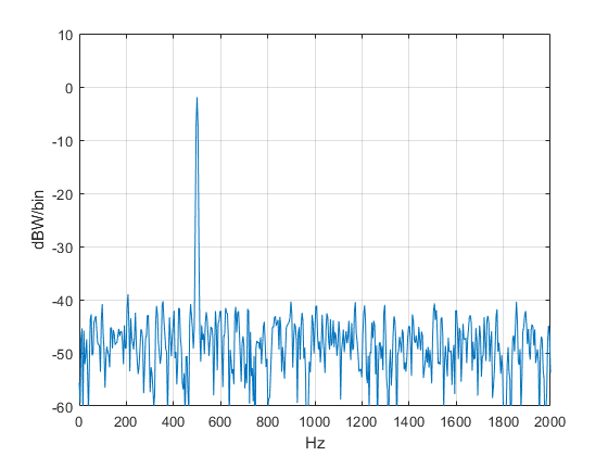
Figure 1.  PSD of sine + noise without DFT averaging.

Example 2.

This example performs DFT averaging.  The signal is the same as example 1, except the number of time samples is increased eight-fold.

    fs= 4000;            % Hz sample rate
    Ts= 1/fs;
    f0= 500;             % Hz sine frequency
    A= sqrt(2);          % V sine amplitude for P= 1 W into 1 ohm.
    nfft= 1024;
    N= nfft*8;           % number of samples in time signal
    n= 0:N-1;            % time index
    x= A*sin(2*pi*f0*n*Ts) + .1*randn(1,N);
    [PdB,f]= psd_simple(x,nfft,fs);

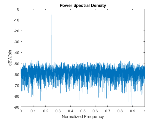
With N = 8*nfft, the function finds the DFT of 15 overlapping 1024-point segments of x, then averages the DFT’s.  The PSD is plotted in Figure 2.  DFT averaging has reduced the variance of the noise floor compared to that of Figure 1.

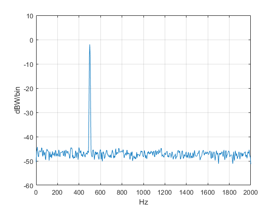
Figure 2.  PSD of sine + noise with DFT averaging.

Choice of Window Function

A window function is usually needed when computing the spectrum of a discrete-time signal [5].  As mentioned, psd_simple uses a Kaiser window function with beta = 7 [3,4].  Figure 3 shows the magnitude response of the Kaiser window, along with that of a Hanning window.  The beta = 7 Kaiser window has the following frequency-domain properties:

noise bandwidth = 1.575 bins

processing loss = 10*log₁₀(noise bw) = 1.97 dB

scallop loss = 1.32 dB

first sidelobe level = -51 dB

For comparison, the Hanning window has processing loss of 1.74 dB and first sidelobe level of -31.5 dB.  I discussed the meaning of these properties in an earlier post [5].

Beta is an adjustable parameter of the Kaiser window.  Larger beta gives lower sidelobe level at the expense of increased noise bandwidth/processing loss.  If you need a different window function, you can just substitute it into the code of psd_simple.

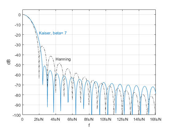
Figure 3.  Magnitude Response of Kaiser window with beta = 7.  N = window length.

Appendix   Matlab Function psd_simple

% function [PdB,f]= psd_simple(x,nfft,fs)  4/13/20 Neil Robertson
% Simple-to-use power spectral density function
% using Welch psd averaging.
%
% x = input signal vector
% nfft = fft length.
% fs = sample frequency, Hz
% PdB = power spectral density, dBW/bin
% f = frequency vector, Hz
%
function [PdB,f]= psd_simple(x,nfft,fs);
noverlap= nfft/2;              % number of overlapped samples
window= kaiser(nfft,7);        % window function
if length(x) < nfft
    N= length(x);
    window= kaiser(N,7);
    noverlap= 0;
end
[pxx,f]= pwelch(x,window,noverlap,nfft,fs);    % W/Hz
PdB= 10*log10(pxx*fs/nfft);                    % convert W/Hz to dBW/bin

References

1.  Robertson, Neil, “Use Matlab Function Pwelch to Find Power Spectral Density – or Do It Yourself”,

https://www.dsprelated.com/showarticle/1221.php

2.  The Mathworks website, https://www.mathworks.com/help/signal/ref/pwelch.html

3.  The Mathworks website, https://www.mathworks.com/help/signal/ug/kaiser-window.html

4.  Oppenheim, Alan V. and Schafer, Ronald W., Discrete-Time Signal Processing, Prentice Hall, 1989,      section 7.4.3.

5.  Robertson, Neil, “Evaluate Window Functions for the Discrete Fourier Transform”, https://www.dsprelated.com/showarticle/1211.php

Neil Robertson        March, 2020

Sign in