


Fractional Delay FIR Filters
Consider the following Finite Impulse Response (FIR) coefficients:
b = [b0 b1 b2 b1 b0]
These coefficients form a 5-tap symmetrical FIR filter having constant group delay [1,2] over 0 to fs/2 of:
D = (ntaps – 1)/2 = 2 samples
For a symmetrical filter with an odd number of taps, the group delay is always an integer number of samples, while for one with an even number of taps, the group delay is always an integer + 0.5 samples. Can we design a filter with arbitrary delay, say 9.3 samples? The answer is yes -- It is possible to design a non-symmetrical FIR filter with arbitrary group delay which is approximately constant over a wide band, with approximately flat magnitude response [3,4]. Let the desired group delay be:
D = (ntaps – 1)/2 + u
= D0 + u samples, (1)
where we call u the fractional delay and -0.5 <= u <= 0.5. D0 is the fixed portion of the total delay; it is determined by ntaps. The appendix lists a simple Matlab function frac_delay_fir.m to compute FIR coefficients for a given value of u and ntaps. The function provides coefficients with approximately flat delay and frequency responses over a frequency range approaching 0 to fs/2.
In this post, we’ll present a couple of examples using the function, then discuss the theory behind it. Finally, we’ll look at an example of a fractional delay lowpass FIR filter with arbitrary cut-off frequency.
Example 1.
This example uses frac_delay_fir.m to compute FIR coefficients for 19-tap filters for several values of u. Starting out with u = 0.3 samples, the group delay from Equation 1 will be approximately:
D = (19 – 1)/2 + 0.3 = 9.3 samples
The following code generates the coefficients, then computes the group delay and magnitude response:
    ntaps= 19;                      % desired number of taps
    u= 0.3;                         % samples desired fractional delay
    b= frac_delay_fir(ntaps,u);     % compute filter coeffs
    [gd,f]= grpdelay(b,1,256,1);    % compute group delay in samples
    [h,f]= freqz(b,1,256,1);        % compute frequency response
    H= 20*log10(abs(h));            % dB magnitude response
The coefficients, along with group delay and magnitude response, are plotted in Figure 1. The group delay and magnitude response are very flat up to about 0.35*fs, with delay of 9.3 samples, as expected.
Figure 4 plots group delay and magnitude response for several values of u. Wider bandwidth could be achieved by increasing the number of taps. For example, a 31-tap filter has flat delay of 15.3 samples up to about 0.41*fs.
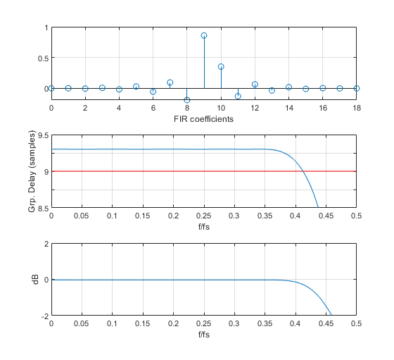
Figure 1. Fractional Delay FIR with ntaps= 19 and u = 0.3 samples
Top: FIR coefficients Middle: Group Delay Response Bottom: Magnitude Response
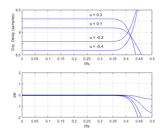
Figure 2. Fractional Delay FIR Filters for ntaps = 19 and several values of u.
Top: Group delay response Bottom: Magnitude response.
Example 2.
This example uses a fractional delay filter to delay or advance a pulse by 0.5 samples. First, we generate a shaped pulse and apply it to a 19-tap FIR with center tap = 1 and all other taps 0. In other words, we are just delaying the pulse by 9 samples. The fractional delay u is 0.
    win= hanning(7)/4;                  % hanning window
    x= conv(win,ones(1,20));            % shaped pulse input
    b_zero= [0 0 0 0 0 0 0 0 0 1 0 0 0 0 0 0 0 0 0];    % filter coeffs, u= 0
    y1= conv(b_zero,x);                 % pulse output for u = 0
The input and output are plotted in Figure 3. Now we’ll delay or advance the pulse by 0.5 samples:
    ntaps= 19;
    b_dly= frac_delay_fir(ntaps,0.5);      % filter coeffs, u= 0.5 samples
    b_adv= frac_delay_fir(ntaps,-0.5);     % filter coeffs, u= -0.5 samples
    y2= conv(b_dly,x);                     % filtered pulse output for u = 0.5
    y3= conv(b_adv,x);                     % filtered pulse output for u = -0.5
The leading edge of the pulses at the FIR output are plotted
in Figure 4 for u= 0, -0.5, and +0.5 samples.
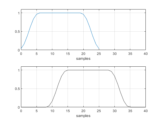
Figure 3. Shaped pulse at input and output of 9-sample delay (ntaps = 19 and u= 0).
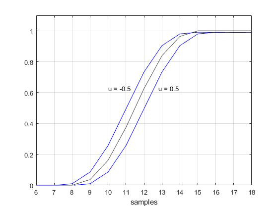
Figure 4. Response of fractional delay filter to a shaped pulse.
ntaps = 19 and u = -0.5, 0, and 0.5 samples.
How it works
The impulse response of an ideal discrete-time lowpass filter with cut-off frequency ωc = 2πfc/fs is [5]:
$$ h(n)=\frac{sin(\omega_c n)}{\pi n} ,\qquad -\infty < n < \infty $$
To delay the response by u samples, where u is a rational
number, we write:
$$ h(n,u)=\frac{sin(\omega_c (n-u))}{\pi (n-u)} ,\qquad -\infty < n < \infty $$
Truncating the response to N + 1 taps, we have:
$$ h(n,u)=\frac{sin(\omega_c (n-u))}{\pi (n-u)} ,\qquad -N/2 < n < N/2 \qquad (2) $$
For a filter with maximum bandwidth, we set fc = fs/2, which gives ωc = π:
$$ h(n,u)=\frac{sin(\pi (n-u))}{\pi (n-u)} ,\qquad -N/2 < n < N/2 \qquad (3) $$
Equation 3 is plotted for u = 0 in the top of Figure 5. The grey line is the continuous function
$sin(\pi(t-u))/(\pi(t-u))$. We can see that for u = 0, Equation 3 reduces to an impulse centered at the middle sample (sample 0). That h(n,u) is an impulse is consistent with our choice of a bandwidth of fs/2. The bottom of Figure 5 shows Equation 3 for u= 0.4. The coefficients now fall on a sinx/x curve that is delayed 0.4 samples, and the response is non-symmetrical. Counting n = 0: N, instead of -N/2 to N/2, the total delay is D0 + u samples (see Equation 1).
To implement a practical filter, we need to multiply h(n,u) in Equation 3 by a window function [6]. Otherwise, truncation to a finite number of taps would produce ripples in both the magnitude and delay responses. The function frac_delay_fir.m uses a Chebyshev window [7,8] with sidelobe level of -70 dB.
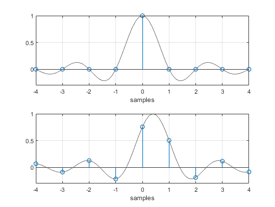
Figure 5. Truncated impulse response of Equation 3 for u = 0 (top) and u = 0.4 (bottom).
The above technique is a variation of the window method of FIR filter design. We could also design the filter by approximation methods in the frequency domain. The desired frequency response is:
$$ H(f)= exp(-j2\pi fDT_s), $$
where Ts is sample time and D is total delay in samples, as defined by Equation 1. Given discrete frequency $f= kf_s/N$, we have:
$$ H(f)= exp(-j2\pi kD/N), \quad k=0:N-1 \qquad (4) $$
It is possible to design the FIR filter using Equation 4 and least-squares or Parks-McClellan approximations [4].
Fractional delay lowpass FIR filters
The function frac_delay_fir.m is based on Equation 3 and has a passband goal of 0 to fs/2 Hz. We can synthesize a fractional delay lowpass filter with arbitrary cut-off frequency by using Equation 2. The filter will have approximately flat delay over most of its passband. A function for this, frac_delay_lpf.m, is listed in the appendix. Note that while frac_delay_fir.m uses a Chebyshev window with -70 dB sidelobes, frac_delay_lpf.m uses a Chebyshev window with -60 dB sidelobes, to avoid a wide transition band in the lowpass response. This results in somewhat higher delay ripple.
Example 3.
This example uses frac_delay_lpf.m to compute FIR coefficients for a 25-tap FIR lowpass filter with fractional delay of 0.4 samples, -6 dB cut-off frequency of 26 Hz, and sample frequency of 100 Hz. Here is the Matlab code to generate the coefficients and compute the group delay and magnitude response:
    ntaps= 25;          % desired number of taps
    fc= 26;             % Hz -6 dB cut-off frequency
    fs= 100;            % Hz sample frequency
    u= 0.4;             % samples desired fractional delay
    %
    b= frac_delay_lpf(ntaps,fc,fs,u);
    [gd,f]= grpdelay(b,1,256,fs);        % compute group delay in samples
    [h,f]= freqz(b,1,256,fs);            % compute frequency response
    H= 20*log10(abs(h));                 % dB magnitude response
Figure 5 plots the filter coefficients, group delay response, and magnitude response. From Equation 1, the group delay in the passband is approximately:
D = (25 – 1)/2 + 0.4 = 12.4 samples
The group delay starts to droop within the filter’s passband; it has decreased by about .06 samples at 20 Hz.
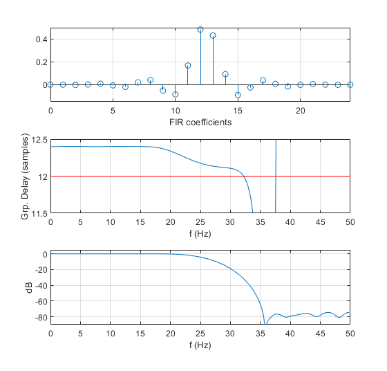
Figure 6. Fractional Delay LPF with ntaps = 25, u = 0.4 samples, fc = 26 Hz, and fs = 100 Hz.
Top: FIR coefficients Middle: Group Delay Response Bottom: Magnitude Response
Appendix Matlab functions for fractional delay FIR filters
The function frac_delay_fir(ntaps,u) has a passband frequency range approaching 0 to fs/2.
The function frac_delay_lpf(ntaps,fc,fs,u) has a programmable -6 dB cut-off frequency fc.
For either function, total delay within the passband is determined by Equation 1, and ntaps may be odd or even. The range of fractional delay u should normally be between -0.5 and 0.5 samples. For |u| > 0.5, the filtered signal is somewhat attenuated because the truncated impulse response 'sinc' is not centered with respect to the window function.
frac_delay_fir.m uses a Chebyshev window with -70 dB sidelobes, while frac_delay_lpf.m uses a Chebyshev window with -60 dB sidelobes, in order to avoid a wide transition band in the lowpass response. This results in somewhat higher delay ripple. You may wish to experiment with different window functions.
    % frac_delay_fir.m 1/29/20 Neil Robertson
    % Fractional delay FIR filter.  Passband range is f= 0 to fs/2.
    %
    % ntaps = number of taps of FIR filter.  ntaps can be odd or even.
    % u = fractional delay in samples.  u can be positive or negative.
    % b = FIR coefficients
    %
    function b= frac_delay_fir(ntaps,u)
    if mod(u,1)== 0
        u= u+ eps;            % eps= 2.2e-16  prevent divide by zero
    end
    N= ntaps-1;
    n= -N/2:N/2;
    sinc= sin(pi*(n-u))./(pi*(n-u));    % truncated impulse response
    win= chebwin(ntaps,70);             % window function
    b= sinc.*win';                      % apply window function
    % frac_delay_lpf.m  2/5/20 Neil Robertson
    % Lowpass FIR filter with fractional delay.
    %
    % ntaps = number of taps of FIR filter. ntaps can be odd or even.
    % u = fractional delay in samples. u can be positive or negative.
    % fc = -6 dB cutoff frequency, Hz
    % fs = sample frequency, Hz
    % b = FIR coefficients
    %
    function b= frac_delay_lpf(ntaps,fc,fs,u)
    if fc/fs > 0.5
        error('fc/fs must be <= 0.5')
    end
    if mod(u,1)== 0
        u= u+ eps;             % eps= 2.2e-16  prevent divide by zero
    end
    wc= 2*pi*fc/fs;
    N= ntaps-1;
    n= -N/2:N/2;
    sinc= sin(wc*(n-u))./(pi*(n-u));    % truncated impulse response
    win= chebwin(ntaps,60);             % window function
    b= sinc.*win';                      % apply window function
References
1. Mitra, Sanjit K., Digital Signal Processing, 2nd Ed.,McGraw-Hill, 2001, p 213 – 214.
2. Lyons, Richard G., Understanding Digital Signal Processing, 3rd Ed., Pearson, 2011, p 897 -898.
3. Javier Diaz-Carmona and Gordana Jovanovic Dolecek (2011). Fractional Delay Digital Filters, Applications of.MATLAB in Science and Engineering, Prof. Tadeusz Michalowski (Ed.), ISBN: 978-953-307-708-6, InTech. http://cdn.intechweb.org/pdfs/18566.pdf
4. Valimaki, Vesa,“[Chapter] 3 Fractional Delay Filters “, http://users.spa.aalto.fi/vpv/publications/vesan_vaitos/ch3_pt1_fir.pdf
5. Mitra, p 448.
6. Mitra, section 7.6.
7. Lyons, Richard, “Computing Chebyshev Window Sequences”, DSP Related website, https://www.dsprelated.com/showarticle/42.php
8. Wikipedia, “Dolph-Chebyshev window”, https://en.wikipedia.org/wiki/Window_function#Dolph%E2%80%93Chebyshev_window
Neil Robertson February, 2020


- Comments
- Write a Comment Select to add a comment
A very well written useful article. Enjoyed reading it.

I'm glad you liked it. Thanks for the feedback.
Neil

Hi Neil. In your interesting blog, thanks for keeping the mathematics tractable!
Rick,
"Tractable" is the only math I know! Math is something that is great when you understand it (or fool yourself that you understand it).
-- Neil
Dear, all
I am working on polynomial Matrix decomposition,
so I need a fractional delay filter (probably, Windowed Sinc function )
to implement 3D (Row x Com. x order of the filter) broadband steering vector.
My problem is I wan to control the delay unit of the fractional delay FIR by myself (to be sin(theta))., and the obtained result to be 3D matrix (M x L x order of FIR)
- function b= frac_delay_FIR(ntaps,u)
- if mod(u,1)== 0
- u= u+ eps; % eps= 2.2e-16 prevent divide by zero,
- end
- N= ntaps-1; % order
- n= -N/2:N/2;
- sinc= sin(pi*(n-u))./(pi*(n-u)); % truncated impulse response
- win= chebwin(ntaps,70); % window function
- b= sinc.*win; % apply window function
My Question is how can I make the result of this Fractional delay filter to be 3D, M x L x Order (Polynomial matrix),?
I highly appreciate your help and advices
Hi,
I don't know anything about polynomial Matrix decomposition. You could try posting your question to the Forum.
regards,
Neil

Nice post, Neil!
I have an observation about the window function you are applying here. It seems to me that the window is a filter itself, and the group delay of the window should be taken into account.
I wasn't sure how to adjust the Chebyshev window to a fractional delay, so I tried comparing the group delay of the filter with the Chebyshev window in your code to a Gaussian window, with and without a fractional delay. Here's the group delay for an 11-tap filter with a fractional delay of 0.5:
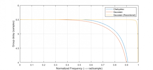
Here's the magnitude response:
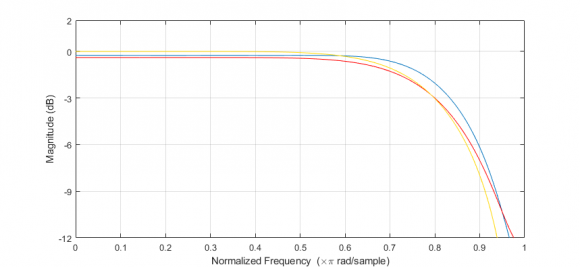
I think it's clear from the plots that the re-centered window with fractional delay gives a much flatter group delay up to very high frequencies. The magnitude response of the Gaussian filter is worse than the Chebyshev filter, but this is a property of the window, not the fractional delay of the window.
Hi pi,
So if I understand you, for an 11-tap filter, with taps b0:b10, I am centering the window at tap b5, regardless of the desired fractional delay. But for your case of fractional delay of 0.5, you are centering the Gaussian window halfway between b5 and b6, which puts it at the center of the truncated
sin(pi(n-.5))./(pi(n-.5)) response.
Neil
Yeah, sounds like you understand what I was trying to say.
I tried my hand at finding a frequency domain justification for it:
Let h(n) be a lowpass filter, and w(n) be the windowing function such that,
x(n) = h(n)w(n),
Then the Fourier transform is given by X(k) = H(k) * W(k).
If we delay h(n) by a value d, then x_1(n)=h(n-d)w(n)
Then the Fourier transform is now X_1(k) = (exp(-jkd)H(k)) * (W(k)), which is not reducible by any clear means (multiplication by a non-scalar doesn't commute with convolution).
However, if we delay both h(n) and w(n) by d, then x(n-d) = h(n-d)w(n-d), the Fourier transform of which is (exp(-jkd)H(k)) * (exp(-jkd)W(k)), which can be shown to equal exp(-jkd)X(k). You may want to evaluate the convolution integral to prove this to yourself.
Have you tested a case other than u = 0.5? What about u = 0.3? Does it perform as well?
-Neil
I really hadn't looked at other fractional delays yet, thanks for directing my attention to that.
Here's a graph showing the group delay with a Gaussian window, with and without the window delay, for fractional delays ranging from 0.1 to 0.5. The standard Gaussian window is shown with the dashed line, while the shifted window is solid.
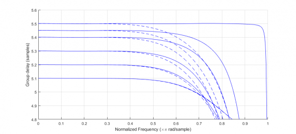
The improvement is certainly less pronounced for the smaller delays, but shifting the window still seems to have a better group delay behavior than keeping the window centered.
Thanks for this detailed reply! One other advantage of shifting the window has to do with signal attenuation. If the window is not shifted, the signal is attenuated slightly as u increases, because the truncated impulse response is not aligned exactly with the window. Shifting the window eliminates the attenuation. This would allow using u values up to a full sample, so you could use 0 < u < 1 instead of -.5 < u < .5.
However, on the whole, it looks like shifting the window will be of limited value.
-- Neil
Hello, Neil Robertson! It's very good article. If you want, you can also insert high-pass modification by change sin by cos, thanks.
Igor,
Thanks for the tip.
Neil

Hello Neil,
Very nice article. Just seen it googling around. I have a question maybe dumb but perhaps you can help. Say I have a delay of 1 unit, followed by a decimation by 2. Can I bring the decimator block in front by using the Nobel identity? This would give 1/2 delay. Does this make any sense?
This is how I got to the point where I needed 1/2 delay and found your article by the way.
Thanks a lot. I hope you still check the blog.
Leo
Hi Leo,
If you can live with some latency, you can make a filter with a delay of, say, exactly 4.5 samples. A symmetrical FIR with length ntaps has delay of
GD = (ntaps - 1)/2.
So, for 4.5 samples delay you could do the following:
fs= 1;
fc= .49;
ntaps= 10;
b= fir1(ntaps-1,2*fc/fs); % lp with fc = .49*fs
[H,f]= freqz(b,1,256,1);
HdB= 20*log10(abs(H));
[GD,f]= grpdelay(b,1,256,1); % group delay in samples
The top plot is the filter coeffs, middle plot is the magnitude response, and bottom plot is the group delay of 4.5 samples. Note I could have used a different value for fc and still gotten a delay of 4.5 samples.
regards,
Neil

Hello again Neil,
Thanks a lot for your answer! I'll just try it all out and let you know how it goes.
Thanks again!
Leo
To post reply to a comment, click on the 'reply' button attached to each comment. To post a new comment (not a reply to a comment) check out the 'Write a Comment' tab at the top of the comments.
Please login (on the right) if you already have an account on this platform.
Otherwise, please use this form to register (free) an join one of the largest online community for Electrical/Embedded/DSP/FPGA/ML engineers: