R1C1R2C2: The Two-Pole Passive RC Filter

I keep running into this circuit every year or two, and need to do the same old calculations, which are kind of tiring. So I figured I’d just write up an article and then I can look it up the next time.

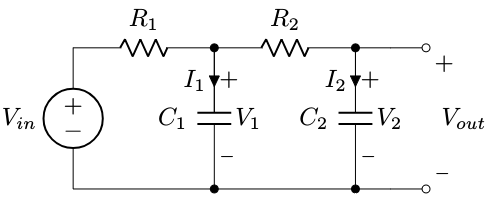
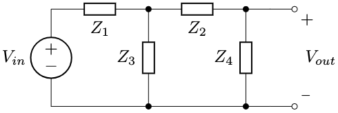
This is a two-pole passive RC filter. Doesn’t work as well as an LC filter or an active filter, but it is cheap. We’re going to find out a couple of things about its transfer function.

First let’s find out the transfer function of this circuit:

Not very difficult:

$$ \frac{V_{out}}{V_{in}} = \frac{Z_4}{Z_2 + Z_4} \cdot \frac{Z_A}{Z_1 + Z_A}$$

where \( Z_A = Z_3 \parallel (Z_2 + Z_4). \)

After a bunch of what I call Grungy Algebra, we get

$$ \frac{V_{out}}{V_{in}} = \frac{Z_3Z_4}{Z_1Z_2 + Z_1Z_3 + Z_1Z_4 + Z_2Z_3 + Z_3Z_4} $$

The problem with Grungy Algebra is that it sows the seeds of Doubt. And we all know that Doubt is bad in engineering. So a couple of ways of double-checking here:

• as \( Z_3 \to 0 \) or \( Z_4 \to 0 \), \( \frac{V_{out}}{V_{in}} \to 0 \)
• as \( Z_3 \to \infty, \frac{V_{out}}{V_{in}} \to Z_4/(Z_1+Z_2+Z_4) \)
• as \( Z_4 \to \infty, \frac{V_{out}}{V_{in}} \to Z_3/(Z_1+Z_3) \)

Numerically:

for Z1, Z2, Z3, Z4 in [(1.0,2.0,3.0,4.0),
                       (4.0,3.0,2.0,1.0),
                       (1.0,10.0,2.0,20.0)]:
    ZA = 1/(1/Z3 + 1/(Z2+Z4))
    print "Z1=%f, Z2=%f, Z3=%f, Z4=%f" % (Z1,Z2,Z3,Z4)
    print "Vo/Vi = Z4ZA/(Z2+Z4)(Z1+ZA) = %f" % (Z4/(Z2+Z4)*ZA/(Z1+ZA))
    print "           = (direct formula) %f" % (Z3*Z4/(Z1*Z2+Z1*Z3+Z1*Z4+Z2*Z3+Z3*Z4))

Z1=1.000000, Z2=2.000000, Z3=3.000000, Z4=4.000000
Vo/Vi = Z4ZA/(Z2+Z4)(Z1+ZA) = 0.444444
           = (direct formula) 0.444444
Z1=4.000000, Z2=3.000000, Z3=2.000000, Z4=1.000000
Vo/Vi = Z4ZA/(Z2+Z4)(Z1+ZA) = 0.062500
           = (direct formula) 0.062500
Z1=1.000000, Z2=10.000000, Z3=2.000000, Z4=20.000000
Vo/Vi = Z4ZA/(Z2+Z4)(Z1+ZA) = 0.434783
           = (direct formula) 0.434783

All looks good!

Now we just need to handle our original circuit.

In this case, \( Z_1=R_1, Z_2=R_2, Z_3=1/sC_1, Z_4=1/sC_2. \) And… we have more Grungy Algebra. After which we get

$$ H(s) = \frac{V_o}{V_i} = \frac{1}{R_1R_2C_1C_2s^2 + R_1C_1s + R_1C_2s + R_2C_2s + 1}$$

More double-checking: if \( C_1=0 \) then we get \( H(s) = \frac{1}{(R_1+R_2)C_2s + 1} \); if \( C_2 = 0 \) then \( H(s) = \frac{1}{R_1C_2s + 1}. \)

A couple of things about this:

For low frequencies, the \( s^2 \) term is very small and \( H(s) \approx \frac{1}{\tau s+1} \) where \( \tau = R_1C_1 + R_1C_2 + R_2C_2 \).

The standard form of the second order system is

$$H(s) = \frac{1}{\tau^2s^2 + 2\zeta\tau s + 1} = \frac{{\omega_n}^2}{s^2 + 2\zeta\omega_n s + {\omega_n}^2}$$

so here we have \( \tau^2 = R_1R_2C_1C_2 \) and \( \zeta = \frac{R_1C_1 + R_1C_2 + R_2C_2}{2\sqrt{R_1R_2C_1C_2}} \)

If \( R_1 = R_2 = R \) and \( C_1 = C_2 = C \), then \( \tau = RC \) and \( \zeta = \frac{3RC}{2RC} = 1.5 \), which is a fairly high damping ratio.

We can get close to a damping ratio of 1 by making the second stage impedances larger; for example if \( R_1 = R, R_2 = kR, C_1 = C, C_2 = \frac{1}{k}C \) then we have \( \tau = RC \) and \( \zeta = \frac{RC + \frac{RC}{k} + RC}{2RC} = 1 + \frac{1}{2k}, \) which means if \( k=10 \) then we get \( \zeta = 1.05. \) We can get close to 1 but we can’t reach it or get below it with this circuit; we’d need inductors or an active filter using transistors or op-amps.

We can also simulate this system using a state-space representation; since currents \( I_1, I_2 \) into the capacitors are \( I_1 = C\frac{dV_1}{dt} = \frac{V_{in} - V_1}{R_1} + \frac{V_2 - V_1}{R_2} \) and \( I_2 = C\frac{dV_2}{dt} = \frac{V_1 - V_2}{R_2}, \) then:

\( \frac{d}{dt}\begin{bmatrix}C_1V_1 \cr C_2V_2\end{bmatrix} = \begin{bmatrix}-\frac{1}{R_1}-\frac{1}{R_2} & \frac{1}{R_2} \cr \frac{1}{R_2} & -\frac{1}{R_2} \end{bmatrix} \begin{bmatrix}V_1 \cr V_2 \end{bmatrix} + \begin{bmatrix}\frac{1}{R_1} \cr 0 \end{bmatrix} V_{in} \)

or

\( \frac{d}{dt}\begin{bmatrix}V_1 \cr V_2\end{bmatrix} = \begin{bmatrix}-\frac{1}{R_1C_1}-\frac{1}{R_2C_1} & \frac{1}{R_2C_1} \cr \frac{1}{R_2C_2} & -\frac{1}{R_2C_2} \end{bmatrix} \begin{bmatrix}V_1 \cr V_2 \end{bmatrix} + \begin{bmatrix}\frac{1}{R_1C_1} \cr 0 \end{bmatrix} V_{in} \)

which is in the canonical state-space form \( \frac{dV}{dt} = AV + Bu \), and we can simulate it with scipy.signal.StateSpace:

import scipy.signal
import matplotlib.pyplot as plt
import numpy as np
%matplotlib inline

C1 = C2 = 0.1e-6
R1 = 1e3
R2 = 10e3
A = np.array([[-1.0/R1/C1-1.0/R2/C1, 1.0/R2/C1],
                          [1.0/R2/C2, -1.0/R2/C2]])
B = np.array([[1.0/R1/C1], [0]])
C = np.array([0,1])
D = 0
ss = scipy.signal.StateSpace(A,B,C,D)

t = np.arange(5000)*1e-6
t, yout, xout = scipy.signal.lsim(ss, t>1e-6, t)
plt.plot(t,yout,'b',label='2nd order system')

tau3 = R1*C1+R1*C2+R2*C2
ss_approx = scipy.signal.StateSpace(-1.0/tau3, 1.0/tau3, 1, 0)

t, yout_approx, xout_approx = scipy.signal.lsim(ss_approx, t>1e-6, t)

plt.plot(t,yout_approx,'r',label='1st order approximation')
plt.xlabel('t')
plt.ylabel('y')
plt.legend(loc='lower right');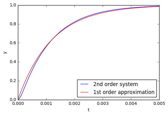

For practical circuit implementations of filters:

• Use NP0/C0G capacitors — these are class 1 ceramic capacitors and are much more ideal than X5R/X7R/Y5V/Z5U capacitors, with lower temperature coefficient, lower tolerances, lower parasitic losses, and less unwanted effects like microphony.
• Don’t use resistors that are too small or too large. Too small of a resistor can load down the input; too large of a resistor can make the output high enough impedance to allow noise to couple into the circuit. The range 1KΩ - 1MΩ is what you will find most often.
• Don’t use capacitors that are too small or too large. Too small of a capacitor may be too high impedance; too large of a capacitor will cost a lot. The range 10pF - 1μF is what you will find most often.
• Low-pass filters with cutoff frequencies of 10Hz or less are difficult to design in analog, and you are probably better off using DSP techniques to filter out any lower frequency content.

And that’s about all there is to say on the subject.

© 2018 Jason M. Sachs, all rights reserved.

Sign in