


Take Control of Noise with Spectral Averaging
Most engineers have seen the moment-to-moment fluctuations that are common with instantaneous measurements of a supposedly steady spectrum. You can see these fluctuations in magnitude and phase for each frequency bin of your spectrogram. Although major variations are certainly reason for concern, recall that we don’t live in an ideal, noise-free world. After verifying the integrity of your measurement setup by checking connections, sensors, wiring, and the like, you might conclude that the variation you see is the result of noise.
Realizing that you cannot eliminate noise, you next set about trying to reduce its influence. If you are building a custom measurement system, you have a number of software options for the job. This article discusses how to reduce spectral noise with different types of averaging, a digital signal processing (DSP) technique.
Averaging is DSP
Most measurement and automation development software ship with ready-to-use DSP routines, for noise reduction and many other tasks. For instance, LabVIEW ships with software tools for both digital filtering and spectral averaging. Although you can easily apply such tools, I’m not advocating blind “black-box” style application—an understanding of what’s under the hood will tell you when and how to apply them. Further, the term “DSP” shouldn’t scare you. If you are looking at a spectrum on a PC-based display, you are likely already using some DSP. Most contemporary dynamic signal analyzers rely on what is perhaps the most famous DSP algorithm, the Fast Fourier Transform (FFT), to calculate the frequency-domain representation (spectrum) from samples of a time domain signal.
The basic idea of averaging for spectral noise reduction is the same as arithmetic averaging to find a mean value. A simple case is time-domain averaging over groups of samples. This operation is a type of low-pass filtering that can reduce high frequency noise. Such filtering is a topic that we will discuss in more detail in the next column.
Spectral averaging is a different approach and is a type of ensemble averaging, which means that the “sample” and “mean value” are both spectra. The “mean value” spectrum results from averaging “sample” spectra. It isn’t quite that simple though, because of the nature of the spectra. When you apply an FFT or another discrete Fourier transform routine to a set of real-world samples to find a spectrum, the output is a set of complex numbers that represent the magnitude and phase of this spectrum.
Software generally stores a spectrum in an array with elements that include the real and imaginary components of each complex number. These elements are samples of spectral estimates with positions in the array (the index) that correspond to particular frequencies. If you are familiar with spectrum analyzer terminology, you can think of each array as a trace with each position in the array representing a particular frequency.
Calculating an average spectrum involves averaging across common frequencies in multiple spectra. Consider an example in which you have collected five time-domain signals and calculated the spectrum for each by applying an FFT. To find each frequency of the averaged spectra, you average across the five corresponding frequencies of your sample spectra.
Vector and RMS Averaging
Because we are working with complex numbers that represent the phase and magnitude of your signal, there are several options for exactly how you perform an average. If you take the square root of the average of the squares of your sample spectra, you are doing RMS Averaging. Another alternative is Vector Averaging in which you average the real and complex components separately. As shown in Fig 1, each reduces noise differently.
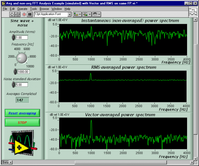
Fig 1. The difference between non-averaged and averaged spectra is clearly visible in these power spectra of a simulated 1kHz triggered sine tone with superimposed white noise. As shown in the top graph, which is a non-averaged spectra, it is difficult to distinguish the peak of this tone above the noise. The bottom two graphs show the results of RMS (middle) and Vector (bottom) averaging of 147 spectra. Notice the reduced variance of the RMS average and the reduced noise floor (but no reduced fluctuation) of the Vector average
The result of RMS averaging is an estimate of the spectrum that contains the same amount of energy as the source. It preserves an estimate of the amount of energy in both the noise and the non-noise signal components of your spectrum.
Just what is the benefit of a process that preserves noise energy? Although RMS averaging preserves noise energy, it reduces the variance (noise fluctuation) in the spectrum. This reduction can distinguish non-noise components and facilitates measurement of the noise floor itself. (This approach is similar to Bartlett's method, which takes its name from the researcher who first studied it extensively. See Ref 1, Section 11.6.3 for more information.)
Vector averaging can actually reduce the noise energy of your spectrum. It does so by averaging the real and complex components separately, which means that the result is an average over both phase and magnitude. This type of averaging causes random phase to cancel out and is equivalent to time-domain averaging. Because you want to reduce only noise, you must make sure that the non-noise portion of your signal doesn’t vary in phase relative to your other sample spectra. This requirement means that the input spectra must share a common non-noise trigger. Put another way, the non-noise components of your input signal(s) must arrive at the averaging stage with the same phase.
Just how close am I?
In applying either vector or RMS averaging, you are essentially trading measurement time for noise control. With either, increasing the number of averaged spectra improves the noise control. The downside is that it takes more time to gather and calculate these spectra.
You can quantify the relationship between the number of sample spectra and reduction of noise with statistics. (To be specific, we are applying averaging in order to find a point estimate of the mean of a population of spectra. The expectation value of this mean is a biased version of the true spectra.) A measure of how far our sample-based mean is from the true mean is its standard error:


Compensating for trends
Our discussion so far assumes that the interesting (non-noise) frequencies of your sample spectra doesn’t change with time and that the noise portion is a stationary, white noise signal with a mean value of zero. If you are acquiring data for immediate analysis and presentation, you have to wonder what happens if the non-noise portion of your spectra changes during acquisition.
To answer this question, consider that online spectral averaging continuously adjusts a display based on an average over some record of previous spectra. With this technique, you continuously update your analysis by averaging in recently acquired spectra with a buffer of older spectra. As such, any change during this process to the interesting (non-noise) portion of your signal will cause older non-noise portions of the signal to average out with the noise. The effect is that newer interesting spectral components appear to rise up out of the noise floor, while older ones sink.
Although you cannot altogether avoid such “in-between” readings due to this effect, you can control the reaction time of your analysis and display by applying a weighting function. With such functions, you can alter the significance (in terms of averaging) to recently acquired spectra relative to older spectra (Fig 2). One option is to assign equal weighting to all spectra, new and old. Such linear weighting is useful for accurate measurements. An alternative is exponential weighting, which applies a greater weight to more recent samples. By adjusting a time-constant associated with this function, you can modify the reaction time of your analysis and display.
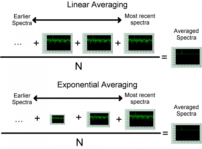
Fig 2. By assigning a weighting function to your average, you can choose between measurement-quality results and display reaction time. Linear weighting (top) assigns equal significance to all spectra in the average, making it slow to react to changes but useful for measurement. With exponential weighting, newer samples carry more significance, which means that you will see changes more quickly if you are monitoring a live display.
With spectral averaging, you have several power tools for spectral noise control. RMS averaging reduces noise fluctuation, which is the variance of your signal due to noise. It doesn’t modify the noise power of the signal, which means that the noise floor remains in place. Vector averaging actually reduces the noise floor. Equivalent to time-domain averaging, vector averaging requires triggered input signals. One trade-off for the benefits for either type of average is your measurement time because the noise control of averaging increases with the number of averages.
The author would like to thank Mike Cerna and Thierry Debelle at National Instruments for their valuable assistance with this article.
References
- Oppenheim, Alan, and Schafer, R., Discrete-Time Signal Processing, Prentice-Hall, Inc. 1989, ISBN 0-13-216292-X.
- Walpole, Robert E. and Myers, R., Probability and Statistics for Engineers and Scientists, 4ed. Macmillan Pub Co., 1989, ISBN 0-02-424210-1.
- White, Robert A., Spectrum and Network Measurements, Prentice-Hall PTR, Inc., 1993, ISBN 0-13-030800-5.


- Comments
- Write a Comment Select to add a comment

Hello Sam. I liked your Figure 2 that used variable-sized rectangles. It's a neat graphical way to show that later spectra (large rectangles) affect the resulting "averaged spectra" more than do earlier spectra (small rectangles).
Hey Sam,
Really interesting article, thanks for sharing.
I have a question that I would like to ask. It might be quite beginner-like though. Is it possible to perform signal averaging from just the magnitude spectrum of certain signal? Or that would only work if we also know the phase information. In that case, what would be the requirement for the signals to average, regarding phase information?
Thank you

Hi Sam,
Don't you mean just the opposite in Figure 2 for exponential averaging with your graphic? In other words, exponential averaging (or any averaging) should have a smoothing effect and not over-respond to new data. Thus, you would want to weigh the cumulative effect of past input samples more heavily than any one recent sample. In equation form, exponential averaging is,
y(n) = a*x(n) + (1-a)*y(n-1), where x(n) is the input, y(n) is the average at index n, and 0 < a < 1.
As one sample example if a = 0.1, then
y(n) = 0.1*x(n) + 0.9*y(n-1).
Admittedly, you could reverse a and (1-a) in the above equation but this is not common in practice as it doesn't provide much smoothing. If you want the best of both worlds, i.e. fast response times and excellent smoothing, then some form of dual mode averaging is required but that's a separate topic.
There is also an explanation of exponential averaging with graphic here on dsprelated by Rick Lyons, link below.
https://www.dsprelated.com/showarticle/72.php
To post reply to a comment, click on the 'reply' button attached to each comment. To post a new comment (not a reply to a comment) check out the 'Write a Comment' tab at the top of the comments.
Please login (on the right) if you already have an account on this platform.
Otherwise, please use this form to register (free) an join one of the largest online community for Electrical/Embedded/DSP/FPGA/ML engineers: