Coefficients of Cascaded Discrete-Time Systems

In this article, we’ll show how to compute the coefficients that result when you cascade discrete-time systems.  With the coefficients in hand, it’s then easy to compute the time or frequency response.  The computation presented here can also be used to find coefficients of mixed discrete-time and continuous-time systems, by using a discrete time model of the continuous-time portion [1].

This article is available in PDF format for easy printing.

Consider the cascade of two systems, H₁(z) and H₂(z), where

$$H_1(z)=K_1\frac{b_0+b_1z^{-1}+...+b_Nz^{-N}}{1+a_1z^{-1}+...+a_Nz^{-N}} = K_1\frac{b_0z^N+b_1z^{N-1}+...+b_N}{z^N+a_1z^{N-1}+...+a_N }$$

$$H_2(z)=K_2\frac{d_0+d_1z^{-1}+...+d_Mz^{-M}}{1+c_1z^{-1}+...+c_Mz^{-M}} = K_2\frac{d_0z^M+d_1z^{M-1}+...+d_M}{z^M+c_1z^{M-1}+...+c_M }$$

H₁(z) and H₂(z) are assumed to have the same sample rate.  H(z) = H₁(z)H₂(z) can be found by multiplying-out the numerator and denominator polynomials of H₁ and H₂.  This can be done by hand, but it turns out there is a rule for multiplying polynomials [2].  The rule is as follows:  Given two polynomials with coefficients b = [b₀ b₁ … b_n] and d = [d₀ d₁ … d_n], the coefficients of the product of the polynomials are given by the convolution of b and d.Thus H(z) = H₁(z)H₂(z) has coefficients:

numerator coeffs = b ⊛ d            (1)

denominator coeffs = a ⊛ c        (2)

where ⊛ indicates convolution.  The overall gain constant is K₁K₂.  For FIR systems, the denominator is unity, so the coefficients of the cascaded systems are b⊛d (which is perhaps no surprise).

Example

Here we’ll cascade 2^nd-order lowpass and band-reject IIR filters with transfer functions H₁(z) and H₂(z) as follows:

$$H_1(z)=K_1\frac{b_0+b_1z^{-1}+b_2z^{-2}}{1+a_1z^{-1}+a_2z^{-2}} $$

where H₁(z) is lowpass with

    a= [1 .3695 .1958]
    b= [1 2 1]
    K1= .3913

$$H_2(z)=K_2\frac{d_0+d_1z^{-1}+d_2z^{-2}}{1+c_1z^{-1}+c_2z^{-2}} $$

where H₂(z) is band-reject with

    c= [1 -1.1074 .8841]
    d= [1 -1.1756 1]
    K2= .942

The frequency responses of the two filters are computed using Matlab as follows:

    fs= 100;                       % Hz sample frequency
    [h1,f]= freqz(K1*b,a,2048,fs);
    H1= 20*log10(abs(h1));         % dB magnitude response
    [h2,f]= freqz(K2*d,c,2048,fs);
    H2= 20*log10(abs(h2));         % dB magnitude response

The responses are plotted in Figure 1.  The cascade coefficients are computed using Equations 1 and 2:

    bb= conv(b,d)
    aa= conv(a,c)
    K= K1*K2

This gives coefficients:

    aa =   1.0000   -0.7379    0.6707    0.1098    0.1731
    bb =   1.0000    0.8244   -0.3512    0.8244    1.0000
    K =    0.3686

The length of aa is 5, so the cascade transfer function is 4^th order.  The transfer function is:

$$H(z)=K\frac{bb_0+bb_1z^{-1}+bb_2z^{-2}+bb_3z^{-3}+bb_4z^{-4}}{1+aa_1z^{-1}+aa_2z^{-2}+aa_3z^{-3}+aa_4z^{-4}} $$

(I apologize for the ungainly notation).  The frequency response is:

    [h,f]= freqz(K*bb,aa,2048,fs);
    H= 20*log10(abs(h));           % dB magnitude response

The cascaded response is shown in the lower plot of Figure 1.

In case you are interested, the lowpass and band-reject coefficients were calculated using the following Matlab code:

    fs= 100;
    fc= 30;
    [b,a]= butter(2,2*fc/fs)         % lowpass coeffs
    f0= 15;
    fU= 16;
    [d,c]= br_synth1(1,f0,fU,fs)     % band-reject coeffs

Here, br_synth1 is a Matlab function developed in an earlier post [3].

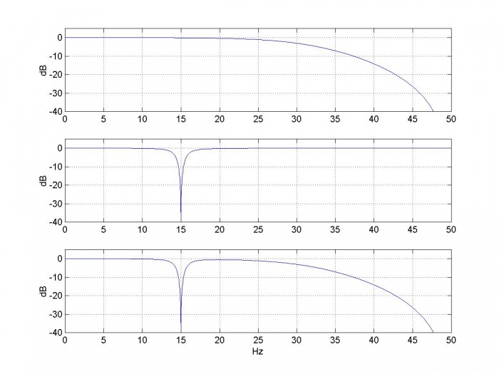
Figure 1.  Magnitude response of cascaded lowpass and Band-reject filters.

top:  Lowpass response |H₁|    middle:  Band-reject response |H₂|    bottom:  cascade response

Neil Robertson            March, 2018

Appendix      Convolution Formulas

The output y[n] of an FIR filter is the discrete convolution of its coefficients b with an input x[n].  We call each of these terms a “sequence”.  Discrete convolution is defined as [4]:

$$y[n]=\sum_{k=-\infty}^{\infty}b[k]\cdot x[n-k]$$

$$=\sum_{k=0}^N b[k]\cdot x[n-k]$$

where N= length(b)-1 and indices of x that are negative or greater than length(x)-1 are ignored.

Cascading two FIR filters uses the same convolution formula.  However, the two sequences are the coefficients of the filters.  When multiplying polynomials, the two sequences are the polynomial coefficients.  In these cases, since we are not dealing with an input signal x, we replace x with another symbol.  Thus the convolution of two discrete sequences b and d is:

$$y[n]=\sum_{k=0}^N b[k]\cdot d[n-k]$$

Where, again, N= length(b)-1.  Convolution is commutative, so we can also write the above equation as:

$$y[n]=\sum_{k=0}^M d[k]\cdot b[n-k]$$

where M= length(d)-1.

References

1.Robertson, Neil, https://www.dsprelated.com/showarticle/1055.php

2.Smith, Julius O., Mathematics of the Discrete Fourier Transform (DFT), https://www.dsprelated.com/freebooks/mdft/Polynomial_Multiplication.html

3.Robertson, Neil, https://www.dsprelated.com/showarticle/1131.php

4.Lyons, Richard G., Understanding Digital Signal Processing, 2^nd Ed., Prentice Hall, 2004, section 5.9.1.

Sign in