


Design IIR Band-Reject Filters
In this post, I show how to design IIR Butterworth band-reject filters, and provide two Matlab functions for band-reject filter synthesis. Earlier posts covered IIR Butterworth lowpass [1] and bandpass [2] filters. Here, the function br_synth1.m designs band-reject filters based on null frequency and upper -3 dB frequency, while br_synth2.m designs them based on lower and upper -3 dB frequencies. I’ll discuss the differences between the two approaches later in this article. Here is an example function call to br_synth1.m:
N= 2;       % order of prototype LPF
f0= 15;     % Hz Null frequency
fU= 16;     % Hz fU= upper -3 dB freq
fs= 100;    % Hz sample frequency
[b,a]= br_synth1(N,f0,fU,fs)
b =    0.9167   -2.1554    3.1004   -2.1554    0.9167
a =    1.0000   -2.2492    3.0935   -2.0616    0.8404
There are five “b” (numerator) and five “a” (denominator) coefficients, so H(z) is 4th order. The frequency response is computed as follows, and is plotted in Figure 1.
[h,f]= freqz(b,a,4096,fs);
H= 20*log10(abs(h));
This article is available in PDF format for easy printing.
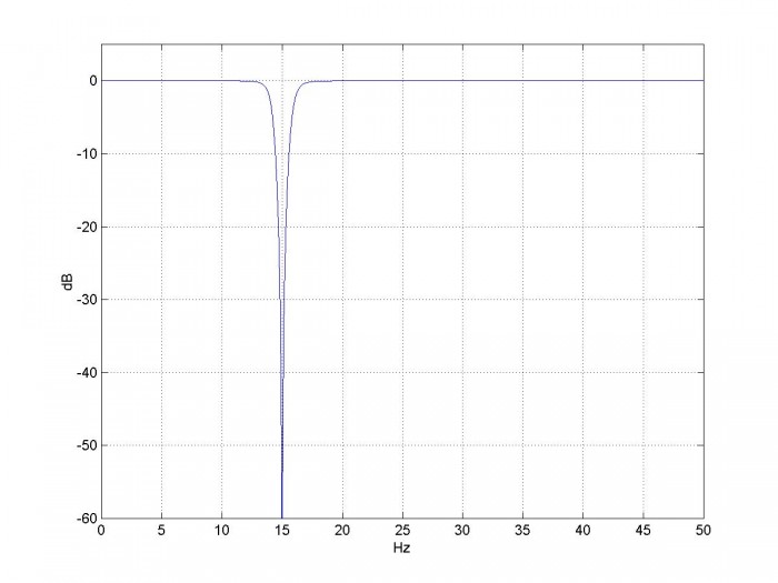
Figure 1. Magnitude response of band-reject filter based on N= 2 lowpass prototype.
f0= 15 Hz, fU= 16 Hz, and fs= 100 Hz.
Filter Synthesis
Here is a summary of the steps for computing the band-reject filter coefficients. Note F is continuous (analog) frequency in Hz and Ω is continuous radian frequency.
- Find the poles of a lowpass analog prototype filter with Ωc = 1 rad/s.
- Given the null frequency f0 and upper -3 dB frequency fU of the digital band-reject filter, find the corresponding frequencies of the analog band-reject filter (pre-warping).
- Transform the analog lowpass poles to analog band-reject poles.
- Transform the poles from the s-plane to the z-plane, using the bilinear transform.
- Add N zeros at z= exp(jω0) and N zeros at z= z= exp(-jω0), where N is the order of the lowpass prototype.
- Convert poles and zeros to polynomials with coefficients an and bn.
These steps are similar to the bandpass design procedure, with steps 2, 3, 5, and 6 modified for the band-reject case. Now let’s look at the design procedure in detail. The Matlab function br_synth1.m that performs the filter synthesis is provided in Appendix A.
1. Poles of the analog lowpass prototype filter. For a Butterworth filter of order N with Ωc = 1 rad/s, the poles are given by [3,4]:
$$p'_{ak}= -sin(\theta)+jcos(\theta)$$
where $$\theta=\frac{(2k-1)\pi}{2N},\quad k=1:N$$
Here we use a prime superscript on p to distinguish the lowpass prototype poles from the yet to be calculated band-reject poles.
2. Given null frequency f0 and upper -3 dB frequency fU of the digital band-reject filter, find the corresponding frequencies of the analog band-reject filter. As before, we’ll adjust (pre-warp) the analog frequencies to take the nonlinearity of the bilinear transform into account:
$$F_0=\frac{f_s}{\pi}tan\left(\frac{\pi f_0}{f_s}\right)$$
$$F_U=\frac{f_s}{\pi}tan\left(\frac{\pi f_U}{f_s}\right)$$
We also need to find the lower -3 dB frequency FL and the bandwidth BWHz:
$F_L=F_0^2/F_U$
$BW_{Hz}=F_U-F_L$
3. Transform the analog lowpass poles to analog band-reject poles. See Appendix B for a derivation of the transformation. For each lowpass pole pa' , we get two band-reject poles:
$$p_a=2\pi F_0\left[\frac{BW_{Hz}}{2F_0p'_a} \pm
j\sqrt{1-\left(\frac{BW_{Hz}}{2F_0p'_a}\right)^2}\ \right]$$
4. Transform the poles from the s-plane to the z-plane, using the bilinear transform (Note there are 2N poles). This is the same as for the IIR bandpass:
$$p_k=\frac{1+p_{ak}/(2f_s)}{1-p_{ak}/(2f_s)},\quad k=1:2N$$
5. Add N zeros on the unit circle at z= exp(jω0) and N zeros at z= exp(-jω0), where ω0= 2πf0/fs. See Appendix B for details. We can now write H(z) as:
$$H(z)=K\frac{(z- e^{j\omega_0})^N(z-e^{-j\omega_0})^N}{(z-p_1)(z-p_2)...(z-p_{2N})}\qquad(1)$$
In br_synth1.m, we represent the N zeros at exp(jω0) and N zeros at exp(-jω0) as a vector:
q= [exp(j*w0)*ones(1,N) exp(-j*w0)*ones(1,N)];
6. Convert poles and zeros to polynomials with coefficients an and bn. If we expand the numerator and denominator of equation 1 and divide numerator and denominator by z2N, we get polynomials in z-n:
$$H(z)=K\frac{b_0+b_1z^{-1}+...+b_{2N}z^{-2N}}{1+a_1z^{-1}+...+a_{2N}z^{-2N}}\qquad(2)$$
The Matlab code to perform the expansion is:
    a= poly(p)
    a= real(a)
    b= poly(q)
    b= real(b)
We want H(z) to have a gain of 1 at ω= 0. Letting z= ejω, we have z= 1. Then, referring to equation 2, we have gain at ω= 0 of:
$$H(z=1)=K\frac{\sum b}{\sum a}$$
So, for gain of 1 at ω= 0, we make $K=\sum a/\sum b$.
Example 1
Let’s repeat the example of Figure 1, adding some more detail. We’ll plot the poles and zeros computed by br_synth1.m, and we’ll also look at the group delay. (Note the pole and zero values are not printed by the code listed in Appendix A). Repeating the function call from above:
N= 2;       % order of prototype LPF
f0= 15;     % Hz Null frequency
fU= 16;     % Hz fU= upper -3 dB freq
fs= 100;    % Hz sample frequency
[b,a]= br_synth1(N,f0,fU,fs)
Here are the poles and zeros:
p = 0.5968 + 0.7504i   0.5278 + 0.7973i   0.5278 - 0.7973i   0.5968 - 0.7504i
q = 0.5878 + 0.8090i   0.5878 + 0.8090i   0.5878 - 0.8090i   0.5878 - 0.8090i
The zeros are on the unit circle, with N= 2 zeros at exp(jω0) and 2 zeros at exp(-jω0). The poles and zeros are plotted in Figure 2. Now let’s look at the filter coefficients.
Numerator coefficients before scaling (note symmetry with respect to center):
b = 1.0000 -2.3511 3.3820 -2.3511 1.0000
Numerator scale factor:
K = 0.9167
Filter coefficients b and a:
    b =    0.9167   -2.1554    3.1004   -2.1554    0.9167
    a =    1.0000   -2.2492    3.0935   -2.0616    0.8404
From K, b, and a, we can write the filter’s transfer function:
$$H(z)=.9167*\frac{1-2.3511z^{-1}+3.382z^{-2}-2.3511z^{-3}+z^{-4}}{1-2.2492z^{-1}+3.0935z^{-2}-2.0616z^{-3}+.8404z^{-4}}$$
The magnitude response was plotted in Figure
1. Figure 3 shows the magnitude and group
delay responses over a 10 Hz bandwidth centered at the null frequency. The group delay response is not very flat,
even outside the -1 dB frequency of the amplitude response.
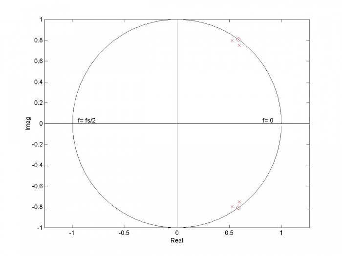
Figure 2. Poles and zeros of band-reject filter based on 2nd order lowpass prototype.
f0= 15 Hz, fU= 16 Hz, and fs= 100 Hz. Zeros at z= exp(+-jω0) are 2nd order.
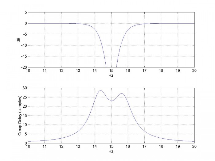
Figure 3. Response of band-reject filter based on 2nd order lowpass prototype.
f0= 15 Hz, fU= 16 Hz, and fs= 100 Hz.
Top: Magnitude Response Bottom: Group Delay [gd,f]= grpdelay(b,a,4096,fs);
Example 2
Let’s look at the magnitude response for different filter orders, for a null frequency f0= 30 MHz and -3 dB bandwidth bw of about 4 Hz. For a narrowband filter, the -3 dB frequencies fU and fL are approximately f0 + bw/2 and f0 - bw/2, respectively. So we have fU= 30 + 2 = 32 Hz. The function call is:
[b,a]= br_synth1(N,f0,fU,fs)
Letting N = 1, 2, and 3, we compute the magnitude response and obtain the plots shown in Figure 4. All of the plots have fU of exactly 32 Hz and fL of slightly less than 28 Hz.
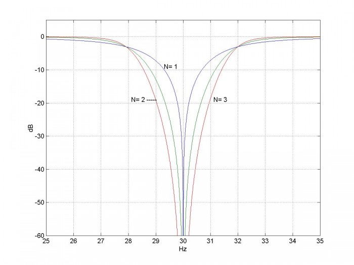
Figure 4. Magnitude response of band-reject filters vs. order of lowpass prototype.
f0= 30 Hz, fU= 32 Hz, and fs= 100 Hz.
Comparing the two Matlab functions for Band-reject Filter Synthesis
From Appendix B, the null frequency of the analog band-reject filter is:
$$\Omega_0=\sqrt{\Omega_L\Omega_U}\qquad(3)$$
where ΩL and ΩH are the lower and upper -3 dB frequencies. In designing a filter, we can choose two of the three parameters in Equation 3, and the other is then determined. For br_synth1.m, we chose Ω0 and ΩH, while for br_synth2.m, we chose ΩL and ΩH. The disadvantage of the latter choice is that the null frequency falls at the geometric mean of ΩL and ΩH, which is not convenient if we want a deep null at a particular frequency.
Figure 5 compares the responses for the two functions. The top plot is for br_synth1.m, with f0= 30 and fU= 34. The bottom plot is for br_synth2.m, with fL= 26 and fU= 34, which results in a null frequency of 30.168 Hz. Table 1 shows how each Matlab function computes frequencies.
Table 1. Frequency Computations of br_synth1.m and br_synth2.m
|
br_synth1(N,f0,fU,fs) |
br_synth2(N,fL,fU,fs) |
|
|
discrete input frequencies |
f0, fU |
fL, fU |
|
Analog pre-warped frequencies |
F0= fs/pi * tan(pi*f0/fs) FU= fs/pi * tan(pi*fU/fs) FL= F0^2/FU
|
FL= fs/pi * tan(pi*fL/fs) FU= fs/pi * tan(pi*fU/fs) F0= sqrt(FL*FU); |
|
resulting discrete frequencies |
fL= fs/pi*atan(pi*FL/fs) |
f0= fs/pi*atan(pi*F0/fs) |
Note that [b,a]= br_synth2(N,fL,fU,fs) gives the same results as the Matlab function
[b,a]= butter(N,[fL fU]*2/fs,’stop’).
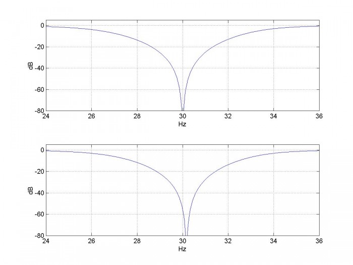
Figure 5. Magnitude Responses of two Matlab functions, fs= 100 Hz
Top: [b,a]= br_synth1(2,30,34,fs)
Bottom: [b,a]= br_synth2(2,26,34,fs)
Coefficient Quantization and Null Depth
The frequency response of a digital filter is H(ejω), with 0 < ω < 2π. In other words, we evaluate H(z) on the unit circle. As shown in Figure 2, a band-reject filter has N zeros at exp(jω0) and N zeros at exp(-jω0), which produce a null in the response at ω0. For a real-world filter, the numerator coefficients b are quantized, which means the zeros don’t fall exactly at the desired spots on the unit circle. As a result, a practical band-reject filter does not have a perfect null at ω0.
Let’s look at how quantization of the numerator coefficients affects the response of the filter in Example 1, which is based on an N= 2 lowpass prototype. Repeating the function call once again:
N= 2;       % order of prototype LPF
f0= 15;     % Hz Null frequency
fU= 16;     % Hz fU= upper -3 dB freq
fs= 100;    % Hz sample frequency
[b,a]= br_synth1(N,f0,fU,fs);
The numerator coefficients are: b = 0.9167 -2.1554 3.1004 -2.1554 0.9167
Now let’s quantize the numerator coefficients to 213 = 8192 steps per unit of coefficient amplitude:
bq= round(b*8192)/8192;
The poles and zeros are then:
q= roots(bq);
p= roots(a);
The amplitude response is computed using bq and a:
[h,f]= freqz(bq,a,Nfft,fs);
H= 20*log10(abs(h));
The resulting zeros and amplitude response are shown in the top row of Figure 6. In the pole-zero plot, which shows just quadrant 1 of the z-plane, you can just notice that the two zeros do not fall at exactly the same place. The depth of the null is about 45 dB. If we quantize to 4096 steps, we get the plots in the bottom row of Figure 6. Null depth is about 33 dB.
Quantizing to 2048 steps gives a null depth of only 25 dB, as shown in the top row of Figure 7. One way to get a deeper null without adding coefficient bits is to experiment with slight offsets of f0, which may result in quantized zero locations that are closer to a point on the unit circle. For example, the bottom row of Figure 7 has 2048 steps and f0 = 15.03 Hz, resulting in a null depth of about 43 dB.
For lowpass prototype N >2 (band-reject order > 4), the effects of quantization of both numerator and denominator coefficients are more pronounced. Quantization of denominator coefficients can cause a pole to move outside the unit circle, making the filter unstable. In many cases, it may be advisable to break the filter up into a cascade of second order sections [5,6].
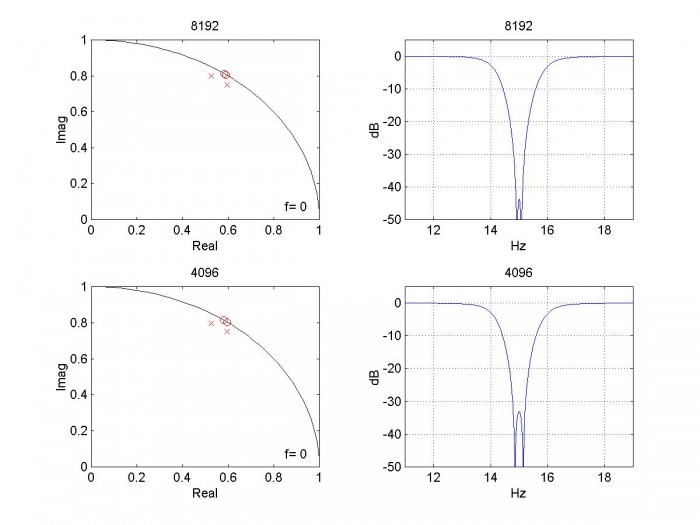
Figure 6. Quantization of numerator coefficients of BRF based on N= 2 lowpass.
Top row: quantization with 8192 steps per unit of coefficient amplitude
Bottom row: quantization with 4096 steps per unit of coefficient amplitude
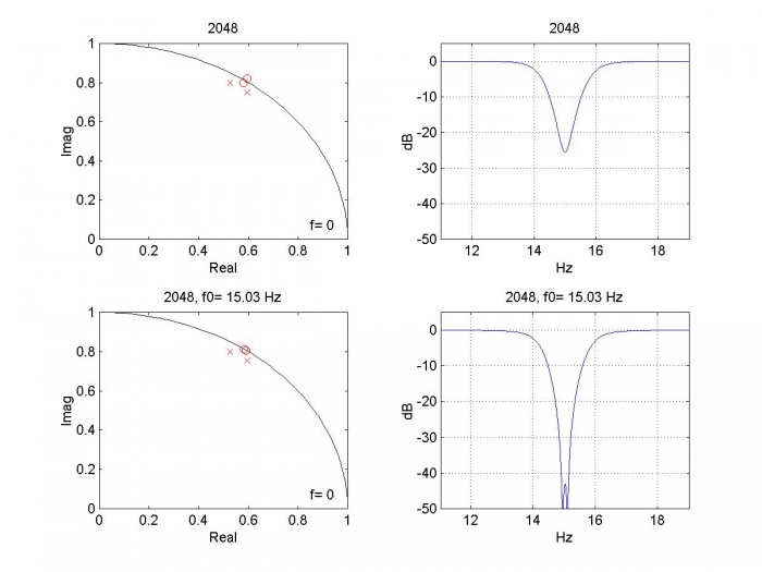
Figure 7. Quantization of numerator coefficients of BRF based on N= 2 lowpass.
Top row: quantization with 2048 steps per unit of coefficient amplitude
Bottom row: quantization with 2048 steps with f0 offset to 15.03 Hz
Appendix A. Matlab Functions br_synth1.m and br_synth2.m
These programs are provided as-is without any guarantees or warranty. The author is not responsible for any damage or losses of any kind caused by the use or misuse of the programs.
%function [b,a]= br_synth1(N,f0,fU,fs)         1/15/18 Neil Robertson
% synthesize band reject IIR Butterworth filter with null frequency f0 and
% upper -3 dB frequency fU.
%
% N= order of prototype LPF
% f0= null frequency, Hz
% fU= upper -3 dB frequency, Hz
% fs= sample frequency, Hz
function [b,a]= br_synth1(N,f0,fU,fs)
if fU>=fs/2
   error('fU must be less than fs/2')
end
% pre-warp f0 and fu
F0= fs/pi * tan(pi*f0/fs);
FU= fs/pi * tan(pi*fU/fs);
FL= F0^2/FU;                  % Hz  analog lower -3 dB freq
BW_hz= FU-FL;                 % Hz analog -3 dB bandwidth
%fL= fs/pi*atan(pi*FL/fs)     % lower -3 dB freq
% find poles of butterworth lpf with Wc = 1 rad/s
k= 1:N;
theta= (2*k -1)*pi/(2*N);
p_lp= -sin(theta) + j*cos(theta);
% transform poles for brf centered at 2*pi*F0
%  note:  alpha and beta are vectors of length N; pa is a vector of length 2N
alpha= BW_hz/F0 * 1 ./(2*p_lp);
beta= sqrt(1- (BW_hz/F0./(2*p_lp)).^2);
pa= 2*pi*F0*[alpha+j*beta  alpha-j*beta];
% find poles and zeros of digital filter
p= (1 + pa/(2*fs))./(1 - pa/(2*fs));         % poles from bilinear transform
w0= 2*pi*f0/fs;
q= [exp(j*w0)*ones(1,N) exp(-j*w0)*ones(1,N)];   % zeros at w0 on unit circle
% convert poles and zeros to numerator and denominator polynomials
a= poly(p);
a= real(a);
b= poly(q);
b= real(b);
% scale coeffs so amplitude is 1.0 at f= 0
K= sum(a)/sum(b);
b= K*b;
%function [b,a]= br_synth2(N,fL,fU,fs)      1/15/18 Neil Robertson
% synthesize band reject IIR Butterworth filter with -3 dB frequencies fL and
%fU.   Note null frequency f0 is offset from center frequency.
%
% N= order of prototype LPF
% fL= lower -3 dB freq, Hz
% fU= upper -3 dB freq, Hz
% fs= sample frequency, Hz
function [b,a]= br_synth2(N,fL,fU,fs)
if fU>=fs/2
   error('fU must be less than fs/2')
end
% pre-warp fL and fU
FL= fs/pi * tan(pi*fL/fs);
FU= fs/pi * tan(pi*fU/fs);
BW_hz= FU-FL;                 % Hz analog -3 dB bandwidth
F0= sqrt(FL*FU);              % Hz analog null frequency
f0= fs/pi*atan(pi*F0/fs);     % Hz discrete null frequency
% find poles of butterworth lpf with Wc = 1 rad/s
k= 1:N;
theta= (2*k -1)*pi/(2*N);
p_lp= -sin(theta) + j*cos(theta);
% transform poles for brf centered at 2*pi*F0
%  note:  alpha and beta are vectors of length N; pa is a vector of length 2N
alpha= BW_hz/F0 * 1 ./(2*p_lp);
beta= sqrt(1- (BW_hz/F0./(2*p_lp)).^2);
pa= 2*pi*F0*[alpha+j*beta  alpha-j*beta];
% find poles and zeros of digital filter
p= (1 + pa/(2*fs))./(1 - pa/(2*fs));         % poles from bilinear transform
w0= 2*pi*f0/fs;
q= [exp(j*w0)*ones(1,N) exp(-j*w0)*ones(1,N)];   % zeros at w0 on unit circle
% convert poles and zeros to numerator and denominator polynomials
a= poly(p);
a= real(a);
b= poly(q);
b= real(b);
% scale coeffs for gain of 1 at f= 0
K= sum(a)/sum(b);
b= K*b;
Appendix B. Lowpass to Band-reject Frequency Transformation
The lowpass to band-reject transformation is the inverse of the lowpass to bandpass transformation we performed in the last post. In the s-domain, we want to transform a normalized lowpass filter with -3 dB frequency of 1 rad/s to a band-reject filter with a given bandwidth and null frequency [7,8]. Once we have the band-reject H(s), we can use the bilinear transform to obtain H(z). We define two frequency variables:
Ω = Im(s) imaginary part of the complex frequency
Ω’ = Im(s’) imaginary part of the normalized complex frequency
(As in the previous two posts, we use Ω for continuous frequency and reserve ω for discrete frequency). To transform H(s’) into H(s), substitute the following for s’:
$$s'=\frac{BW}{\Omega_0} \frac{1}{\left(\frac{s}{\Omega_0}+\frac{\Omega_0}{s}\right)}\qquad B-1$$
where BW = ΩU-ΩL = -3 dB bandwidth and $\Omega_0=\sqrt{\Omega_L\Omega_U}$. As we will show, Ω0 is the null frequency of the filter. Rearranging B-1, we have:
$$s'=BW\frac{s}{s_2+\Omega_0^2}\qquad B-2$$
Then, solving for s:
$$s=\Omega_0\left[\frac{BW}{2\Omega_0s'} \pm j\sqrt{1-\left(\frac{BW}{2\Omega_0s'}\right)^2}\ \right]$$
If we replace s’ with a normalized lowpass pole location pa’, we have:
$$p_a=\Omega_0\left[\frac{BW}{2\Omega_0p'_a} \pm j\sqrt{1-\left(\frac{BW}{2\Omega_0p'_a}\right)^2}\ \right]\qquad B-3$$
For each lowpass pole pa’ , we get two band-reject poles. Thus if the lowpass filter has order N, H(s) for the band-reject filter has order 2N. The IIR filter’s poles are computed from pa using the bilinear transform, as discussed in step 4 in the section on filter synthesis.
For the Matlab function, we replace Ω0 with 2πF0 and replace BW with 2π*BWHz:
$$p_a=2\pi F_0\left[\frac{BW_{Hz}}{2F_0p'_a} \pm j\sqrt{1-\left(\frac{BW_{Hz}}{2F_0p'_a}\right)^2}\ \right]\qquad B-4$$
Oddly enough, the poles of Butterworth band-reject and band-pass filters with the same order, center frequency and bandwidth are identical. (This results from the lowpass prototype complex-conjugate poles falling on a unit circle in the s-plane). Thus the feedback (denominator) coefficients of the bandpass and band-reject filters are the same.
Zeros of H(s) and H(z)
Consider a single-pole normalized lowpass transfer function in s’:
$$H(s')=\frac{1}{s'-\alpha}$$
It has a zero at s’= infinity. From B-2, we have for the corresponding
band-reject filter:
$$H(s)=\frac{1}{BW\frac{s}{s_2+\Omega_0^2}-\alpha}$$
$$H(s)=\frac{s^2+\Omega_0^2}{BW*s-\alpha(s^2+\Omega_0^2)}$$
$$H(s)=\frac{(s+j\Omega_0)(s-j\Omega_0)}{BW*s-\alpha(s^2+\Omega_0^2)}$$
H(s) has zeros at +jΩ0 and - jΩ0. In general, if H(s’) has N zeros at infinity, then H(s) has N zeros at +jΩ0 and N zeros at - jΩ0. Thus Ω0 is the null frequency of the analog band-reject filter.
In the z-domain, H(z) has zeros on the unit circle at exp(jω0) and exp(-jω0), where ω0 is related to Ω0 by the frequency mapping of the bilinear transform [1]:
$$\Omega_0=2f_stan(\omega_0/2)$$
or
$$\omega_0=2tan^{-1}\left(\frac{\Omega_0}{2f_s}\right)$$
We can now write H(z) in pole-zero format
as:
$$H(z)=K\frac{(z- e^{j\omega_0})^N(z-e^{-j\omega_0})^N}{(z-p_1)(z-p_2)...(z-p_{2N})}\qquad B-5$$
A z-plane pole-zero plot illustrating the zeros on the unit circle is shown in Example 1 in the main text (Figure 2).
In the Matlab functions br_synth1.m and br_synth2.m, we expand the numerator and denominator of H(z) to get the filter coefficients. Note you can begin to expand the numerator by hand as follows:
$$numerator=[z^2-z(e^{j\omega_0} +e^{-j\omega_0})+1]^N$$
$$=[z^2-2cos(\omega_0)z+1]^N$$
It then turns out that the numerator
coefficients are symmetric with respect to the center coefficient, and the
first and last coefficients are unity (before scaling by K).
Appendix C Notation
Notation for normalized lowpass continuous frequencies:
normalized radian frequency Ω’ rad/s
normalized complex frequency s’= σ + jΩ’
Notation for band-reject filter continuous frequencies:
-3 dB frequencies ΩL , ΩU rad/s
-3 dB bandwidth BW rad/s
null frequency $\Omega_0=\sqrt{\Omega_L\Omega_U}$ rad/s
- 3 dB bandwidth, Hz BWHz Hz
null frequency, Hz F0 Hz
Notation for band-reject filter discrete frequencies:
-3 dB frequencies, Hz fL , fU Hz
null frequency, Hz f0 Hz
General notation:
continuous frequency F Hz
continuous radian frequency Ω radians/s
complex frequency s = σ + jΩ
discrete frequency f Hz
discrete normalized radian frequency ω = 2πf/fsradians, where fs = sample frequency
Finally, the Matlab functions represent the -3 dB continuous bandwidth (Hz) as BW_hz.
References
1. Robertson, Neil , “Design IIR Butterworth Filters Using 12 Lines of Code”, Dec 2017 https://www.dsprelated.com/showarticle/1119.php
2. Robertson, Neil , “Design IIR Bandpass Filters”, Jan 2017 https://www.dsprelated.com/showarticle/1128.php
3. Williams, Arthur B. and Taylor, Fred J., Electronic Filter Design Handbook, 3rd Ed., McGraw-Hill, 1995, section 2.3
4. Analog Devices Mini Tutorial MT-224, 2012 http://www.analog.com/media/en/training-seminars/tutorials/MT-224.pdf
5. Oppenheim, Alan V. and Shafer, Ronald W., Discrete-Time Signal Processing, Prentice Hall, 1989, sections 6.8 and 6.9.
6. Lyons, Richard G., Understanding Digital Signal Processing, 2nd Ed., Pearson, 2004, sections 6.7 and 6.8
7. Blinchikoff, Herman J., and Zverev,Anatol I., Filtering in the Time and Frequency Domains, Wiley, 1976, section 4.7.
8. Nagendra Krishnapura , “E4215: Analog Filter Synthesis and Design Frequency Transformation”, 4 Mar. 2003 http://www.ee.iitm.ac.in/~nagendra/E4215/2003/handouts/freq_transformation.pdf
Neil Robertson January, 2018 Revised 4/3/2019


- Comments
- Write a Comment Select to add a comment
Hi Neil,
Fantastic article! I have two questions / comments about your approach here with reference to your article on the design of IIR Bandpass Filters:
1 - dealing with the transformation ( lowpass to band reject ),
2 - dealing with the scaling of the numerator coefficients.
I'm currently working on implementing IIR filters via FPGA's , using cascading BiQuads, Lowpass, Highpass, Bandpass, Bandreject, so your articles have been very helpful.
1. In your Designing IIR Bandpass filters article, your introduce the transformation for transforming a lowpass filter into a bandpass filter by:
s' = Q ( s + 1/s ) , <--- note this is normalized and has not been frequency scaled yet.
and in this article your use the transformation for transforming a lowpass filter to band reject filter by:
s' = 1 / ( Q ( s + 1/s )) <---- note this is also normalized and has not been frequency scaled yet.
What I have found is that you can actually use either transformation for both bandpass and bandreject filter. It would go something like this:
To transform a lowpass to bandpass OR a highpass to bandreject you can use:
s' = Q ( s + 1/s )
To transform a lowpass to bandreject OR a highpass to bandpass you can use:
s' = 1 / ( Q ( s + 1/s ))
In both cases, the math works out the same! I had implemented my bandreject filters using the first method before I had discovered this article, I saw that you were doing it different, so out of curiosity I tweaked my algorithm to implement method two and got the same result. Now being really curious, I tried method two back on my bandpass filters and the results were the same!
2. For my question on scaling, I am going to use an example Band Reject filter with fl = 200Hz, fu = 800 Hz, giving the BW = 600 and the geometric mean = 400, and a Q of 0.66666, N=4. Since I am implementing cascading biQuads, I am concerned about what is happening with each biQuad.
Without implementing any scaling, you can see that frequencies before the notch are symmetrical about 0dB, and frequencies post notch converge to 0dB.
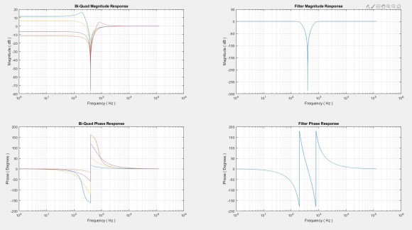
Using your scaling method, you multiply the numerators of each biQuad by the inverse of the DC Gain, ie sum( ak ) / sum( bk ), setting each biQuad's DC gain at 0db. Doing that yeilds:
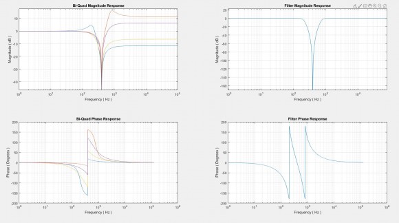
in this case, frequencies pre notch are now scaled at 0dB, but frequencies post notch are now symmetrical about 0dB.
Would a better approach for scaling be to "balance" the frequencies pre and post notch? ie
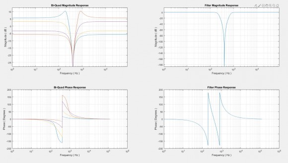
To implement this, I scaled the numerators of each biQuad by ( sum( bk ) / sum( ak ) ) ^(-1/2)
I know this article doesn't really focus on biQuads, but is one approach better than another?
This issue seems to be unique to bandreject filters, and isn't an issue with bandpass filters.
Thanks for putting out good material!
-brandon

Hi Brandon,
I'm glad you liked the post. I have not looked at implementing a BRF using cascaded biquads. As you said, in my post on LP cascaded biquads, each biquad was scaled for gain of 1 at f = 0, and this works for the BRF case as well. I suppose the biquads could also be scaled for gain of 1 at f = fs/2. I don't know if that would have any merit.
regards,
Neil
To post reply to a comment, click on the 'reply' button attached to each comment. To post a new comment (not a reply to a comment) check out the 'Write a Comment' tab at the top of the comments.
Please login (on the right) if you already have an account on this platform.
Otherwise, please use this form to register (free) an join one of the largest online community for Electrical/Embedded/DSP/FPGA/ML engineers: