Design IIR Butterworth Filters Using 12 Lines of Code

While there are plenty of canned functions to design Butterworth IIR filters [1], it’s instructive and not that complicated to design them from scratch.  You can do it in 12 lines of Matlab code.  In this article, we’ll create a Matlab function butter_synth.m to design lowpass Butterworth filters of any order.  Here is an example function call for a 5^th order filter:

N= 5           % Filter order
fc= 10;        % Hz cutoff freq
fs= 100;       % Hz sample freq
[b,a]= butter_synth(N,fc,fs)
    b =    0.0013    0.0064    0.0128    0.0128    0.0064    0.0013
    a =    1.0000   -2.9754    3.8060   -2.5453    0.8811   -0.1254

Then, to find the frequency response:

[h,f]= freqz(b,a,256,fs);
H= 20*log10(abs(h));

The magnitude response of the 5^th order filter is shown in Figure 1, along with the response of the analog prototype.

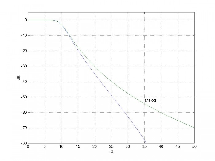
Figure 1.  Magnitude response of N= 5 IIR Butterworth filter with f_c = 10 Hz and f_s = 100 Hz.  The prototype analog filter’s response is also shown.

Notation

First, a word about notation.  We need to distinguish frequency variables in the continuous-time (analog) world from those in the discrete-time world.  In this article, the following notation for frequency will be used:

continuous frequency                                     F  Hz

continuous radian frequency                         Ω  radians/s

complex frequency                                          s = σ + jΩ

discrete frequency                                           f  Hz

discrete normalized radian frequency            ω = 2πf/f_sradians, where f_s = sample freq

Background

Analog Butterworth filters have all-pole transfer functions.  For example, a third-order Butterworth filter with Ω_c = 1 rad/s has the transfer function:

$$H(s)=\frac{1}{s^3+2s^2+2s+1}$$

or

$$H(s)=\frac{1}{(s-p_{a0})(s-p_{a1})(s-p_{a2}) }\qquad(1)$$

where the subscript a denotes analog (s-plane) poles.  The poles in the s-plane are:

 p_a0 =  -.5 + j.866

p_a1 =   -1

p_a2 =   -.5 -j.866

We will transform the poles in the s-plane to poles in the z-plane using the bilinear transform [2,3].  The bilinear transform converts H(s) to H(z) by replacing s with:

$$s=2f_s\frac{1-z^{-1}}{1+z^{-1}}\qquad(2)$$

where f_s is sample frequency.  If we solve for z, we get:

$$z=\frac{1+s/(2f_s)}{1-s/(2f_s)}\qquad(3)$$

Equation 3 maps a point on the s plane to a point on the z plane.  For example, if f_s= 2 Hz, the s-plane real pole at -1 maps to:

$$p=\frac{1-1/4}{1+1/4}=0.6$$

For the 3^rd order filter, with Ω_c=  1 and f_s= 2, the z-plane poles fall as shown in Figure 2.

From equation 1, H(s) has 3 zeros at s= ∞.  How do they map to the z plane?  We will show later that the bilinear transform maps -∞ to ∞ on the jΩ axis  to -f_s/2 to f_s/2 on the unit circle.  So the 3 zeros of H(s) map to +/- f_s/2 on the unit circle, which corresponds to z= -1.  (Recall that on the unit circle, z= e^jω, where ω = 2πf/f_s.  For f = +/-f_s/2, we have ω = +/-π, so z = e^jπ = -1).  The three zeros are represented by the ‘o’ in figure 2.

We can now write the 3^rd-order Butterworth H(z) as:

$$H(z)=K\frac{(z+1)(z+1)(z+1)}{(z-p_0)(z-p_1)(z-p_2)}\qquad(4)$$

where, from equation 3, p= [0.7143 +j 0.33   0.6   0.7143 -j 0.33].  Expanding the numerator and denominator, we have:

$$H(z)=K\frac{b_0z^3+b_1z^2+b_2z+b_3}{z^3+a_1z^2+a_2z+a_3}$$

$$H(z)=K\frac{b_0+b_1z^{-1}+b_2z^{-2}+b_3z^{-3}}{1+a_1z^{-1}+a_2z^{-2}+a_3z^{-3}}\qquad(5)$$

Where b = [1 3 3 1] and a= [1 -2.0286 1.4762 -0.3714].  K is chosen to make gain = 1 at ω= 0:  K = 1/H(ω=0) = 1/H(z=1) = sum(a)/sum(b)= .00952

Looking again at Figure 1, you may have wondered why the attenuation of the IIR filter is greater than that of the analog filter as f approaches f_s/2.  The reason is that the analog filter’s zeros are at ∞, while the bilinear transform compresses the frequency scale so that the IIR filter’s zeros are at f_s/2.

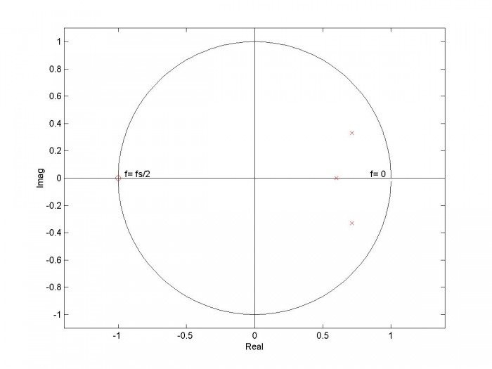
Figure 2.  Z-plane Poles and zeros of 3^rd order IIR Butterworth filter with Ω_c=  1 and f_s= 2.

Filter Synthesis

Here is a summary of the steps for finding the filter coefficients :

1. Find the poles of the analog prototype filter with Ω_c = 1 rad/s.
2. Given the desired f_c of the digital filter, find the corresponding analog frequency F_c.
3. Scale the s-plane poles by 2πF_c.
4. Transform the poles from the s-plane to the z-plane.
5. Add N zeros at z = -1.
6. Convert poles and zeros to polynomials with coefficients a_n and b_n.

Now let’s look at the steps in detail.  Note we’ll repeat a lot of the math we already presented above.  A Matlab function butter_synth that performs the filter synthesis is provided in the Appendix.  It gives the same results as the built-in Matlab function butter(n,Wn) [1].

1.  Poles of the analog filter.  For a Butterworth filter of order N with Ω_c = 1 rad/s, the poles are given by [4,5]:

$$p_{ak}= -sin(\theta)+jcos(\theta)$$

where $$\theta=\frac{(2k-1)\pi}{2N},\quad k=1:N$$

2.  Given the desired f_c, find analog frequency F_c.  As we’ll show in the next section, the bilinear transform does not map the analog frequency F to discrete frequency f linearly.  To achieve a digital filter cut-off frequency of f_c, the analog prototype cut-off frequency must be:

$$F_c=\frac{f_s}{\pi}tan\left(\frac{\pi f_c}{f_s}\right)$$

This exercise is called frequency pre-warping.  For example, if f_s= 100 Hz and we want f_c= 20 Hz, then F_c = 23.13 Hz.

3.  Scale the s-plane poles by 2πF_c. The poles obtained in step 1 gave Ω_c = 1 rad/s (i.e. 1/(2π) Hz).  Multiplying the poles by 2πF_c scales the analog filter cut-off frequency to F_c and the digital filter cut-off frequency to f_c.

4.  Transform the poles from the s-plane to the z-plane using the bilinear transform.  From equation 3,

$$p_k=\frac{1+p_{ak}/(2f_s)}{1-p_{ak}/(2f_s)},\quad k=1:N$$

5.  Add N zeros at z = -1.  Following the example of equation 4, the numerator of H(z) is                (z + 1)^N , meaning there are N poles at z = -1.  We now can write H(z) as:

$$H(z)=K\frac{(z+1)^N}{(z-p_0)(z-p_1)...(z-p_{N-1})}\qquad(6)$$

In butter_synth, we represent the N zeros as a vector q= -ones(1,N).

6.  Convert poles and zeros to polynomials with coefficients a_n and b_n.  If we expand the numerator and denominator of equation 6, we get polynomials in z^-n:

$$H(z)=K\frac{b_0+b_1z^{-1}+...+b_Nz^{-N}}{1+a_1z^{-1}+...+a_Nz^{-N}}\qquad(7)$$

 The Matlab code to perform the expansion is:

a= poly(p)
a= real(a)
b= poly(q)

We want H(z) to have a gain of 1 at ω= 0.  Letting z= e^jω, we have z= 1.  Then, referring to equation 7, we have gain at ω= 0 of:

$$H(z=1)=K\frac{\sum b}{\sum a}$$

So, for gain of 1 at ω= 0, we make $K=\sum a/\sum b$.

And that's the last step.  Figure 3 shows the frequency response vs. order N for filters synthesized by butter_synth.  Figure 4 shows the impulse response vs. order N for three cases.

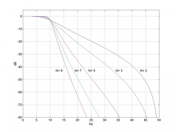
Figure 3.  IIR Butterworth magnitude responses for f_c= 10 Hz and f_s= 100 Hz.

[h,f]= freqz(b,a,256,fs);
H= 20*log10(abs(h));<\pre>

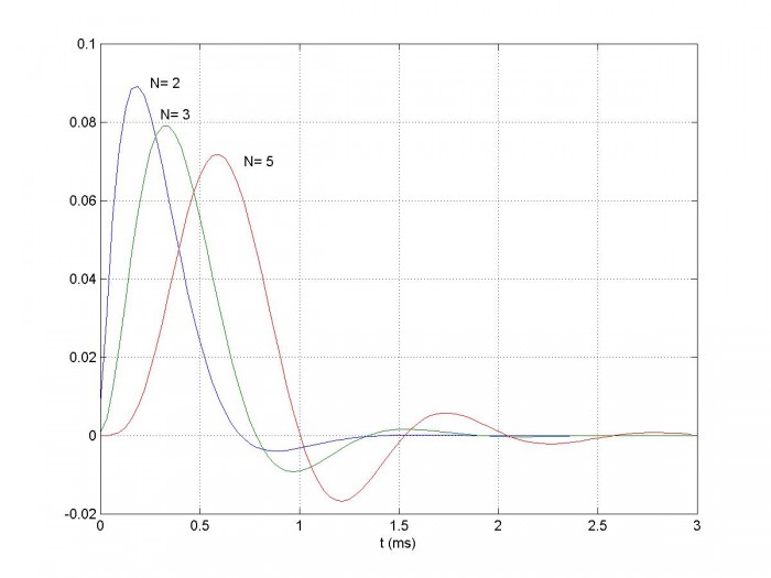
Figure 4.  IIR Butterworth impulse responses for fc = 1 kHz and fs = 32 kHz.

x= [1 zeros(1,95)];  % impulse
y= filter(b,a,x);    % impulse response

Frequency Mapping of the Bilinear Transform

The bilinear transform does not map the continuous frequency F to discrete frequency f linearly.   To show this, we evaluate equation 2 for s= jΩ and z= e^jω:

$$j\Omega=2f_s\frac{1-e^{-j\omega}}{1+e^{-j\omega}}$$

$$j\Omega=j2f_stan(\omega/2)$$

Now substitute Ω= 2πF and ω= 2πf/f_s:

$$F=\frac{f_s}{\pi}tan\left(\frac{\pi f}{f_s}\right)\qquad(8)$$

Figure 5 plots equation 8 for fs= 100 Hz.  The entire analog frequency range maps to  –f_s/2 to f_s/2.  Also shown on the zoomed plot on the right is the transformation of discrete frequency f = 20 Hz to continuous frequency F = 23.13 Hz.  Note that the frequency mapping is approximately linear for f < f_s/10 or so.

Figure 6 shows the effect of using equation 8 to pre-warp the cut-off frequency of an analog prototype filter to give f_c = 20 Hz.  With pre-warping, the analog prototype poles were scaled by 2π*23.13_.  Without pre-warping, they were scaled by 2π*20.

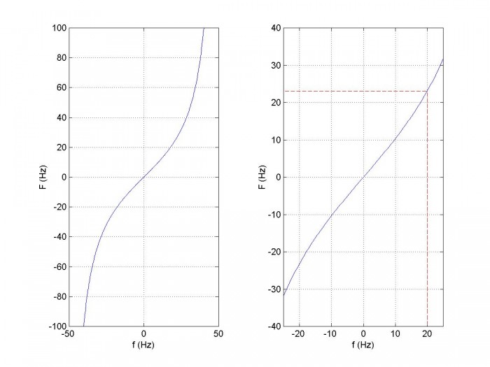
  Figure 5.  Frequency mapping of the bilinear transform for f_s = 100 Hz.  x axis is discrete frequency and y-axis is continuous frequency.  The right plot is a zoomed version of the left plot, showing the value of F for f = 20 Hz.

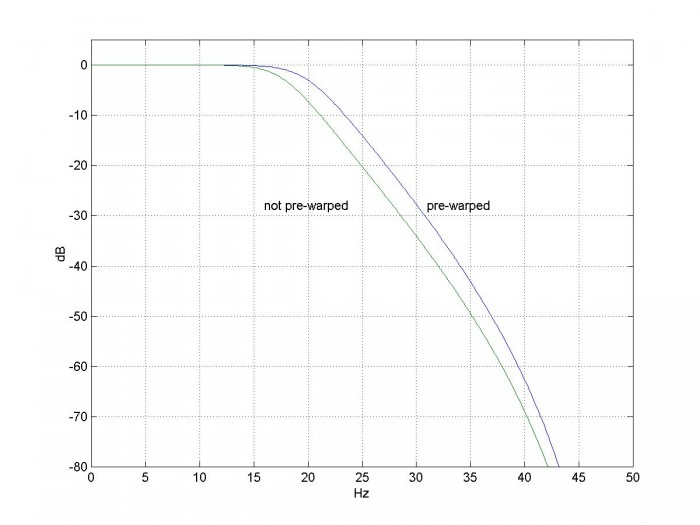
Figure 6.  Effect of pre-warping for f_c = 20 Hz and f_s = 100 Hz.  5^th order IIR Butterworth.

References

1.  Mathworks website https://www.mathworks.com/help/signal/ref/butter.html

2.  Oppenheim, Alan V. and Shafer, Ronald W., Discrete-Time Signal Processing, Prentice Hall, 1989, section 7.1.2

3.  Lyons, Richard G., Understanding Digital Signal Processing, 2^nd Ed., Pearson, 2004, section 6.5

4.  Williams, Arthur B. and Taylor, Fred J., Electronic Filter Design Handbook, 3^rd Ed., McGraw-Hill, 1995, section 2.3

5.  Analog Devices Mini Tutorial MT-224, 2012 http://www.analog.com/media/en/training-seminars/tutorials/MT-224.pdf

Neil Robertson   December 2017

Appendix    Matlab Function butter_synth  (12 lines of code, excluding error check)

This program is provided as-is without any guarantees or warranty.  The author is not responsible for any damage or losses of any kind caused by the use or misuse of the program.

% butter_synth.m    12/9/17 Neil Robertson
% Find the coefficients of an IIR butterworth lowpass filter 
% using bilinear transform
%
% N= filter order
% fc= -3 dB frequency in Hz
% fs= sample frequency in Hz
% b = numerator coefficients of digital filter
% a = denominator coefficients of digital filter
%
function [b,a]= butter_synth(N,fc,fs);
%
if fc>=fs/2;
   error('fc must be less than fs/2')
end
% I.  Find poles of analog filter
k= 1:N;
theta= (2*k -1)*pi/(2*N);
pa= -sin(theta) + j*cos(theta);     % poles of filter with cutoff = 1 rad/s
%
% II.  scale poles in frequency
Fc= fs/pi * tan(pi*fc/fs);          % continuous pre-warped frequency
pa= pa*2*pi*Fc;                     % scale poles by 2*pi*Fc
%
% III.  Find coeffs of digital filter
% poles and zeros in the z plane
p= (1 + pa/(2*fs))./(1 - pa/(2*fs));      % poles by bilinear transform
q= -ones(1,N);                   % zeros
%
% convert poles and zeros to polynomial coeffs
a= poly(p);                   % convert poles to polynomial coeffs a
a= real(a);
b= poly(q);                   % convert zeros to polynomial coeffs b
K= sum(a)/sum(b);             % amplitude scale factor
b= K*b;

Sign in