


There's No End to It -- Matlab Code Plots Frequency Response above the Unit Circle
This post is available in PDF format for easy printing
plotfil3d
Purpose Plot frequency response around the unit circle above the Z-plane.
Syntax
plotfil3d(b,a,N)
plotfil3d(b,a,N,az)
Description
plotfil3d(b,a,N) plots the frequency response magnitude of a digital filter as a 3D curve above the unit circle in the Z-plane. Vertical axis units are dB. The frequency response is computed using the Matlab function freqz(b,a,N,’whole’) as
$$ H(z) = \frac{b(1)+b(2)z^{-1}+b(3)z^{-2}+...}{a(1)+a(2)z^{-1}+a(3)z^{-2}+...}$$
where b and a are the filter coefficient vectors and z = ejω. The response is computed for N values of ω equally spaced over 0 to 2π.
To plot the response for an FIR filter, set a = 1. For efficient computation, N should be chosen as a power of 2.
plotfil3d(b,a,N,az) plots the frequency response as above, except the plot viewing azimuth in degrees is determined by az.
Example 1
Plot the magnitude response of an FIR lowpass filter with cutoff frequency = 0.15*fs.
Compute filter coefficients:
fnorm= .3;                 % fnorm = fc/(fs/2)
b= fir1(30,fnorm);         % window-based FIR coeffs, order = 3
Create a conventional response plot in two dimensions:
N= 512;
[h,f]= freqz(b,1,N,'whole',1);   % freq response
H= 20*log10(abs(h));             % dB freq response
plot(f,H),grid
axis([0 1 -80 5]),xlabel('f/fs'),ylabel('dB')
The 2D plot is shown in Figure 1. Now plot in three dimensions:
plotfil3d(b,1,N); % plot with default viewing azimuth
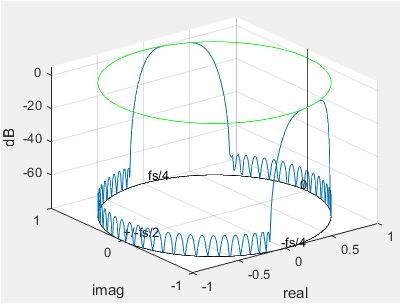
The resulting response, shown in Figure 2, is basically Figure 1 formed into a cylinder. Note that frequency increases in the counter-clockwise direction around the unit circle, so the frequencies from 0 to fs/2 are on the left (although this is not apparent because the response is symmetrical). We can also look at the response from another angle. Using an azimuth of 120 degrees places the frequencies from 0 to fs/2 on the right (Figure 3):
az= 120;                 % degrees azimuth for viewing plot
plotfil3d(b,1,N,az);
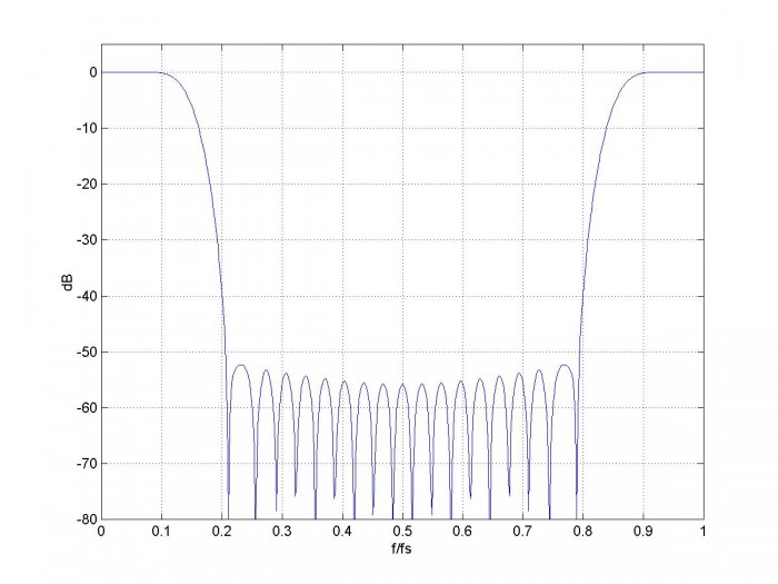
Figure 1. Conventional Plot of magnitude response
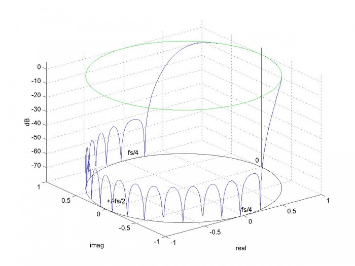
Figure 2. 3D Plot of magnitude response
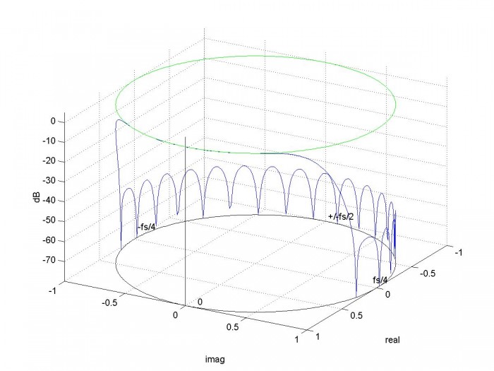 Figure 3. 3D plot with azimuth = 120 degrees
Example 2
Plot the magnitude response of an FIR bandpass filter. Let sample frequency = 200 Hz, lower stopband = 0 to 25 Hz, passband = 37 to 43 Hz, upper stopband = 55 to 100 Hz.
Nfil= 62;                     % filter order
f= [0 25 37 43 55 100]/100;   % define stopband and passband freqs
a = [0 0 1 1 0 0];            % bpf goal function
b= firpm(nfil,f,a);           % synthesis using Parks-McClellan algorithm
N= 512;
plotfil3d(b,1,N)
The response magnitude is shown in Figure 4.
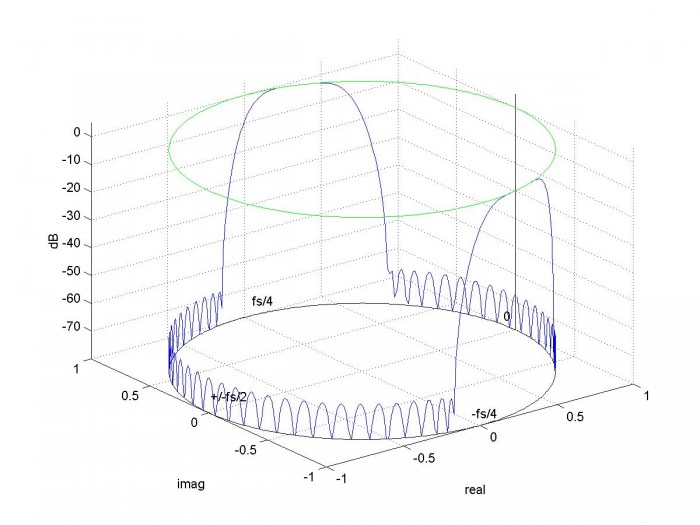
Figure 4. Magnitude response of bandpass FIR filter
Example 3
Plot the magnitude response of a 5th order Butterworth IIR filter with cutoff frequency of 0.08*fs. Plot the filter’s poles and zeros in the Z-plane.
fnorm= .16;                   % fnorm = fc/(fs/2)
[b,a]= butter(5,fnorm);       % synthesize 5th order Butterworth IIR filter
N= 256;
plotfil3d(b,a,N);
q= roots(b)                   % zeros of H(z)
p= roots(a)                   % poles of H(z)
plot3(real(p),imag(p),-80*ones(1,5),'xr')
plot3(real(q),imag(q),-80*ones(1,5),'or')
There are 5 zeros, all near -1 + j0:
q =
  -1.0008
  -1.0003 + 0.0008i
  -1.0003 - 0.0008i
  -0.9993 + 0.0005i
  -0.9993 - 0.0005i
The 5 poles are:
p =
   0.7628 + 0.3988i
   0.7628 - 0.3988i
   0.6306 + 0.2038i
   0.6306 - 0.2038i
   0.5914
The response plot with poles and zeros is shown in Figure 5.
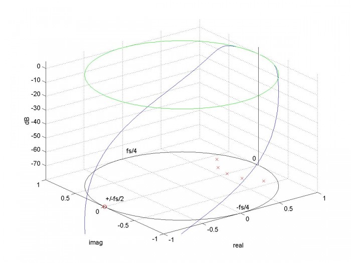
Figure 5. Magnitude response of 5th order Butterworth LP filter, with poles and zeros shown in the Z-plane.
Reference
1. Lyons, Richard, Understanding Digital Signal Processing 2nd Ed., Prentice Hall, 2011, p 288.
Appendix Matlab Function plotfil3d
% plotfil3d.m     10/17/17  revised 11/13/17  Neil Robertson
% Plot Magnitude Response above unit circle in the z-plane
% note w (omega) is defined as w= 2*pi*f/fs = 2*pi*k/N (radians).
% For f= fs/2, w = pi
function plotfil3d(b,a,N,az);
clf
if nargin < 4
   az= -37.5;                    % degrees  default viewing azimuth
end
h = freqz(b,a,N,'whole');        % freq response from 0 to 2*pi
H= 20*log10(abs(h)+eps);   % dB freq response (eps= 2E-16 prevents log of 0)
% unit circle in z-plane
k= 0:N-1;                        % frequency index
w= 2*pi*k/N;                     % radians
z= exp(j*w);                     % unit circle
% plot frequency response and unit circles
H(H<-80)= -80;                   % limit min value of H to -80 dB
plot3(real(z),imag(z),H),grid
view(az,30)                      % use az (degrees) to set viewing azimuth
top= max(H);
hold on
plot3([1 1],[0 0],[top-80 top+5],'k')           % z axis
plot3(real(z),imag(z),(top-80)*ones(1,N),'k')   % unit circle at max(H)-80 dB
plot3(real(z),imag(z),top*ones(1,N),'g')        % unit circle at max(H) dB
xlabel('real'),ylabel('imag'),zlabel('dB')
axis([-1 1 -1 1 top-80 top+5])
% frequency labels
text(1,.1,top-77,'0')
text(.05, 1,top-75,'fs/4')
text(-.95,.05,top-76,'+/-fs/2')
text(-.05, -1,top-75,'-fs/4')


- Comments
- Write a Comment Select to add a comment

Oh come on Neil, you seem bored in your retirement. Many of us can hardly manage the 2D plot. Thanks anyway and at least it proves that 2D is subset of 3D

Kaz,
Yes, I may be getting to the bottom of my shallow well of DSP knowledge!
Neil

Hi Neil. Those plots are neat!
Rick,
Thanks, I'll add you to the list of admirers (so far that's you and my mother).
For some reason, I just find them to be mesmerizing.
Neil
Hi Neil. Yes, please add me to your official list of admirers.
Regarding your 'plotfil3d()' function, you might try thresholding the computed 'H' sequence using:
Threshold = -80; % dB threshold level for specmag plots
H(H<Threshold) = Threshold; % Min dB plot level)>
to see if that makes your plots look even prettier. (Of course you can change that -80 value to some other value.)
Here's your Figure 4 using the -80 (dB) value:
Rick,
Thanks for the suggestion. I updated the post to include this feature.
regards,
Neil
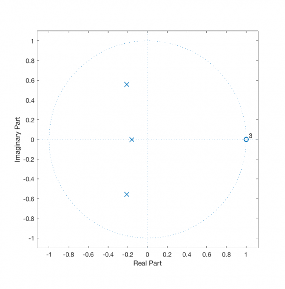
The zplane function could be helpful for visualizing (aspects of) these things as well:
Wn = 300/500;
[b,a] = butter(3,Wn,'high');
zplane(b, a);
My previous post looks like this:
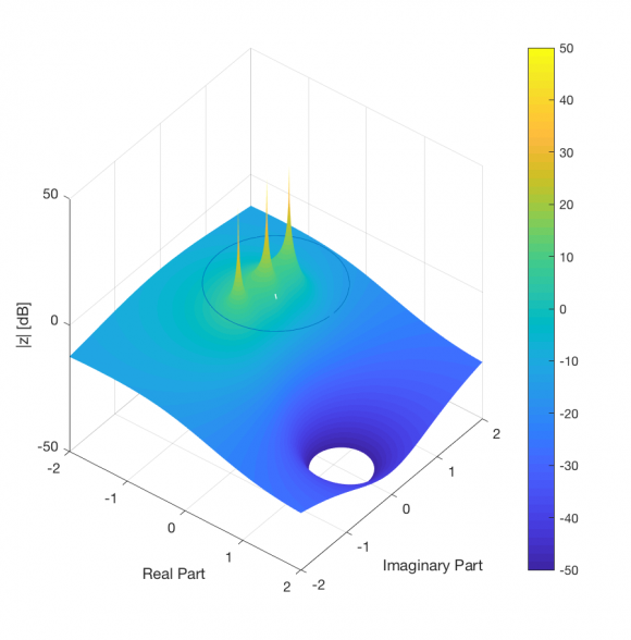
I suppose you could do something ala this as well (my z-plane comprehension is getting rusty at this point):
Wn = 300/500;
N = 3;
[b,a] = butter(3,Wn,'high');
[X, Y] = meshgrid(-2:.01:2, -2:.01:2);
Z = X+1j*Y;
Zev = sum(shiftdim(b, -1) .* Z.^shiftdim(-1:-1:-(N+1), -1), 3) ./ ...
      sum(shiftdim(a, -1) .* Z.^shiftdim(-1:-1:-(N+1), -1), 3);
Nifty, thanks.
Neil
To post reply to a comment, click on the 'reply' button attached to each comment. To post a new comment (not a reply to a comment) check out the 'Write a Comment' tab at the top of the comments.
Please login (on the right) if you already have an account on this platform.
Otherwise, please use this form to register (free) an join one of the largest online community for Electrical/Embedded/DSP/FPGA/ML engineers: